Do I Really Need to Remember All That Stuff Forever? Kalman Filter

Prerequisites

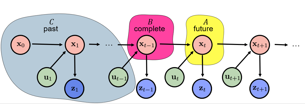
\[\noindent \textbf{Def:} Event \( \mathbf{A} \) is \textit{conditionally independent} on \( \mathbf{C} \) given \( \mathbf{B} \) iff \( p(\mathbf{A} \,|\, \mathbf{B}, \mathbf{C}) = p(\mathbf{A} \,|\, \mathbf{B}) \)\\ \noindent \textbf{Def:} State \( \mathbf{x}_{t-1} \) is \textit{complete} iff future \( \mathbf{x}_t \) is conditionally independent on past given \( \mathbf{x}_{t-1} \)\\ \noindent Consequences: \begin{itemize} \item {State-transition probability:} \begin{equation} p(\mathbf{x}_t | \mathbf{x}_{t-1}, \mathbf{u}_t) = p(\mathbf{x}_t | \mathbf{x}_{t-1}, \mathbf{u}_t, x_{0:t-2}, z_{1:t-1}, u_{1:t-1}) \label{st-pst} \end{equation} \item {Measurement probability:} \begin{equation} p(\mathbf{z}_t | \mathbf{x}_t) = p(\mathbf{z}_t | \mathbf{x}_t, x_{0:t-1}, z_{1:t-1}, u_{1:t}) \label{m-pst} \end{equation} \end{itemize} \begin{figure}[H] \centering \includegraphics[width=0.95\textwidth]{imgs/complete_states.png} \caption{Complete state ilustration.} \label{fig:complete_states} \end{figure}\]

Bayes Filter

The Bayes filter is an algorithm for probabilistic state estimation in dynamic systems. It predicts the state of a system over time, given control inputs and sensory measurements. The filter performs two main steps in a repetitive manner: prediction and measurement update.

\[\begin{itemize} \item \textbf{Initialization:} The belief of the initial state is represented by \( bel(\mathbf{x}_0) \) at time \( t = 1 \). \item \textbf{Prediction Step:} Given the control action \( u_t \) at time \( t \), the prediction step computes a prior belief state: \begin{equation} \overline{\text{bel}}(\mathbf{x}_t) = \int p(\mathbf{x}_t | \mathbf{x}_{t-1}, \mathbf{u}_t) \, \text{bel}(\mathbf{x}_{t-1}) \, d\mathbf{x}_{t-1} \label{bayes-prior} \end{equation} \item \textbf{Measurement Update:} Upon receiving a new measurement \( z_t \), the measurement update refines the predicted belief to produce a posterior belief state: \begin{equation} \text{bel}(\mathbf{x}_t) = \eta \, p(\mathbf{z}_t | \mathbf{x}_t) \, \overline{\text{bel}}(\mathbf{x}_t) \label{bayes-posterior} \end{equation} where \( \eta \) is a normalization constant that ensures the posterior belief is a valid probability distribution by integrating to 1. \end{itemize}\]

Kalman Filter

The Kalman filter is a powerful algorithm used for estimating the state of a system over time. It operates on a simple yet effective principle: predict the future state, then update this prediction with new observations. It handles systems with uncertainties and noise quickly and effectively, making it widely utilized.

Linear System with Gaussian Noise

The Kalman filter assumes a linear system with Gaussian noise.

\[\begin{equation} \mathbf{x}_t = \mathbf{A}_t \mathbf{x}_{t-1} + \mathbf{B}_t \mathbf{u}_t + \mathbf{w}_t \end{equation} \begin{equation} \mathbf{z}_t = \mathbf{C}_t \mathbf{x}_t + \mathbf{v}_t \end{equation} where $\mathbf{A}_t$, $\mathbf{B}_t$, $\mathbf{C}_t$ are matrices that define the system dynamics, $\mathbf{u}_t$ is the control input,~$\mathbf{x}_t$~is~state vector and \( \mathbf{w} \sim \mathcal{N}(0, \mathbf{R}_t) \) and \( \mathbf{v} \sim \mathcal{N}(0, \mathbf{Q}_t) \) are the transition and measurement noise with covariance matrices \( \mathbf{R}_t \) and \( \mathbf{Q}_t \), respectively. This implies that all probability distributions involved are Gaussian, which simplifies computation. The state-transition and measurement probabilities are modeled as follows: \begin{equation} p(\mathbf{x}_t | \mathbf{x}_{t-1}, \mathbf{u}_t) = \mathcal{N}({\mathbf{x}_t};\mathbf{A}_t\mathbf{x}_{t-1} + \mathbf{B}_t\mathbf{u}_t, \mathbf{R}_t) \label{gauss-st-pst} \end{equation} \begin{equation} p(\mathbf{z}_t | \mathbf{x}_t) = \mathcal{N}({\mathbf{z}_t};\mathbf{C}_t\mathbf{x}_t, \mathbf{Q}_t) \label{gauss-meas-pst} \end{equation}\]

Implementation of Kalman Filter

Combining the principles of the Bayes filter (equations \ref{bayes-prior} and \ref{bayes-posterior}), with prerequisities (equations \ref{st-pst} and \ref{m-pst}) and the properties of linear Gaussian systems (equations \ref{gauss-st-pst} and \ref{gauss-meas-pst}), we can derive the Kalman filter update equations:

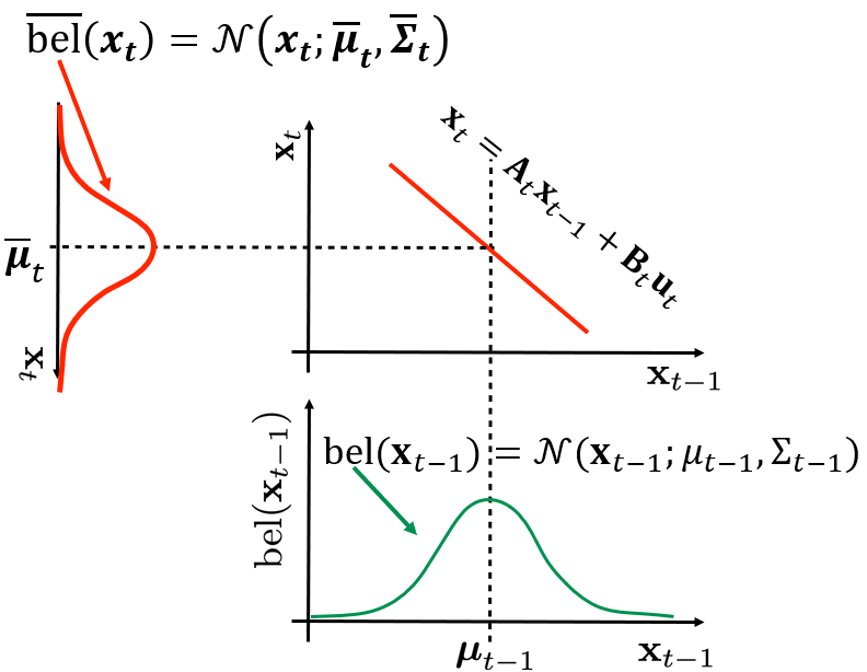
\[\begin{itemize} \item \textbf{Prediction step} (new action \( \mathbf{u}_t \)): \begin{align} \overline{\boldsymbol{\mu}}_t &= \mathbf{A}_t \boldsymbol{\mu}_{t-1} + \mathbf{B}_t \mathbf{u}_t \\ \overline{\boldsymbol{\Sigma}}_t &= \mathbf{A}_t \boldsymbol{\Sigma}_{t-1} \mathbf{A}_t^\top + \mathbf{R}_t \\ \overline{\text{bel}}(\mathbf{x}_t) &= \mathcal{N}({\mathbf{x}_t};\overline{\boldsymbol{\mu}}_t, \overline{\boldsymbol{\Sigma}}_t) \end{align} \item \textbf{Measurement update} (new measurement \( \mathbf{z}_t \)): \begin{align} \mathbf{K}_t &= \overline{\boldsymbol{\Sigma}}_t \mathbf{C}_t^\top (\mathbf{C}_t \overline{\boldsymbol{\Sigma}}_t \mathbf{C}_t^\top + \mathbf{Q}_t)^{-1} \\ \boldsymbol{\mu}_t &= \overline{\boldsymbol{\mu}}_t + \mathbf{K}_t(\mathbf{z}_t - \mathbf{C}_t \overline{\boldsymbol{\mu}}_t) \\ \boldsymbol{\Sigma}_t &= (\mathbf{I} - \mathbf{K}_t \mathbf{C}_t) \overline{\boldsymbol{\Sigma}}_t \\ \text{bel}(\mathbf{x}_t) &= \mathcal{N}({\mathbf{x}_t};\boldsymbol{\mu}_t, \boldsymbol{\Sigma}_t) \end{align} \end{itemize} where \( \boldsymbol{\mu}_t \) is the estimated mean, \( \boldsymbol{\Sigma}_t \) is the estimated uncertainty (covariance), and \( \mathbf{K}_t \) is the Kalman gain which minimizes the estimated uncertainty. In the following picture \ref{fig:predictKF}, we can see the propagation of the state estimate and its uncertainty through a linear function in the prediction step. The \textcolor{mygreen}{Green Gaussian} represents the prior belief, and the \textcolor{myred}{Red Gaussian} represents the posterior belief. \begin{figure}[H] \centering \includegraphics[width=0.6\textwidth]{imgs/predict_intuition_KF.png} \caption{Linear system propagation.} \label{fig:predictKF} \end{figure}\]

Kalman Filter Example: Squeezes Gaussian

\[In this example of a Kalman Filter, the state of a system is represented by position and velocity of the robot. The state can be expressed as a vector $\textbf{x} = \begin{bmatrix} x \\ v \end{bmatrix}$. In this example the state-transition probability is defined as \[ p(\mathbf{x}_t | \mathbf{x}_{t-1}, \mathbf{u}_t) = \mathcal{N} ( \mathbf{x}_t; \underbrace{\begin{bmatrix} 1 & 1 \\ 0 & 1 \end{bmatrix}}_{\mathbf{A}_t} \mathbf{x}_{t-1} + \underbrace{\begin{bmatrix} 1 & 0 \\ 0 & 1 \end{bmatrix}}_{\mathbf{B}_t} \mathbf{u}_t, \underbrace{\begin{bmatrix} 0.01 & 0 \\ 0 & 0.01 \end{bmatrix}}_{\mathbf{R}_t} ) \] and measurement probability is \[ 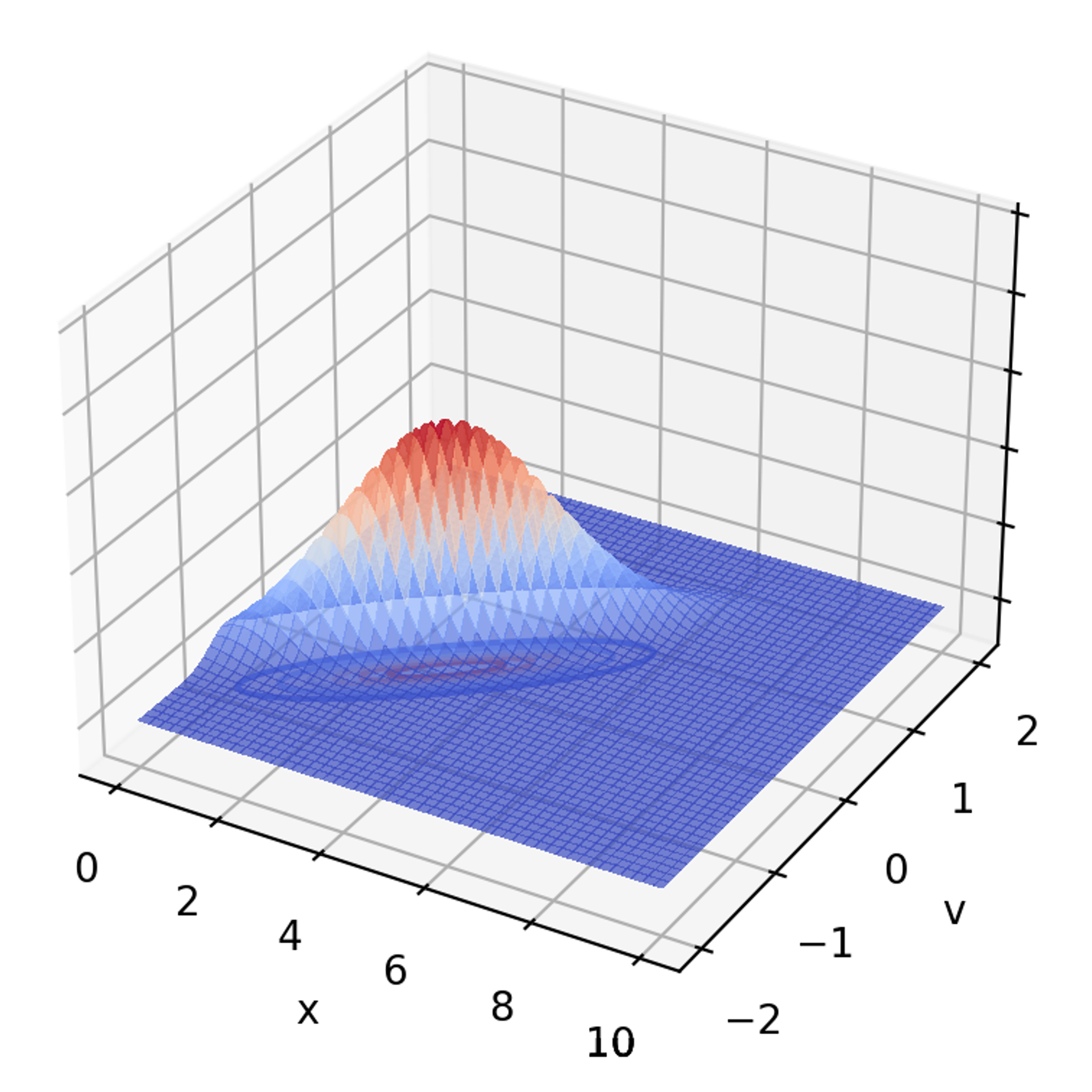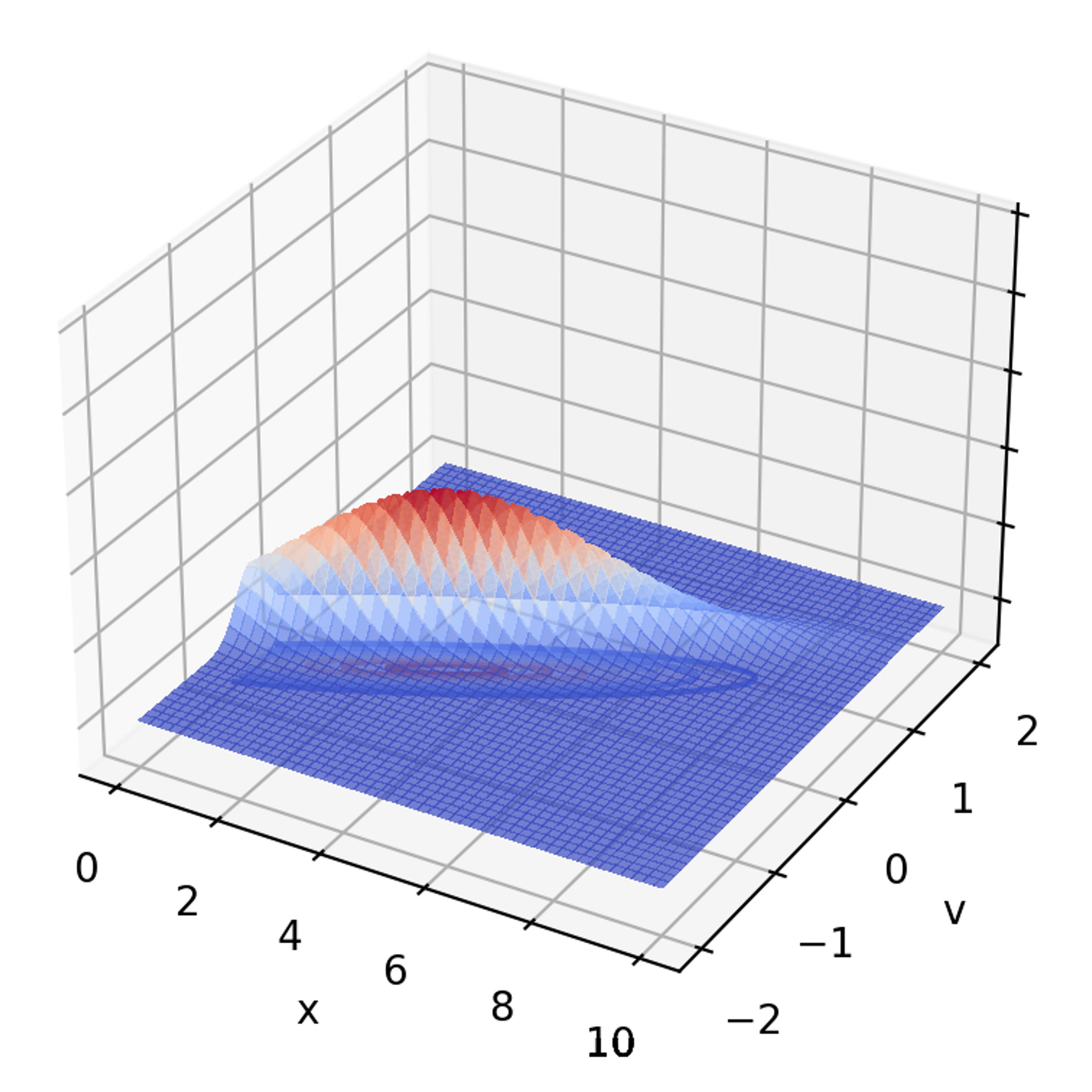p(\mathbf{z}_t | \mathbf{x}_t) = \mathcal{N} ( \mathbf{z}_t; \underbrace{\begin{bmatrix} 1 & 0 \end{bmatrix}}_{\mathbf{C}_t} \mathbf{x}_{t-1}, \underbrace{\begin{bmatrix} 0.3 \end{bmatrix}}_{\mathbf{Q}_t} ) \text{.} \] When there are no measurements available the probability distribution (modeled as a Gaussian) tends to become more squeezed and skewed over time. This is due to the growing uncertainty in predictions as time progresses. Additionally, the skewing of the distribution is caused by the linear dependence of position on velocity. The sequence of images (Figure \ref{fig:squeezing}) demonstrates how the distribution evolves from $x_0$ to $x_5$, visually representing the increasing uncertainty at different time steps. \begin{figure}[H] \centering \begin{subfigure}{0.32\textwidth} \includegraphics[width=\linewidth]{imgs/squeezing_x0.png} \caption{time \(t = 0\)} \label{fig:sq_x0} \end{subfigure} \hfill \begin{subfigure}{0.32\textwidth} \includegraphics[width=\linewidth]{imgs/squeezing_x3.png} \caption{time \(t = 3\)} \label{fig:sq_x3} \end{subfigure} \hfill \begin{subfigure}{0.32\textwidth} \includegraphics[width=\linewidth]{imgs/squeezing_x5.png} \caption{time \(t = 5\)} \label{fig:sq_x5} \end{subfigure} \caption{Visualization of state squeezing and skewing at different time steps.} \label{fig:squeezing} \end{figure} 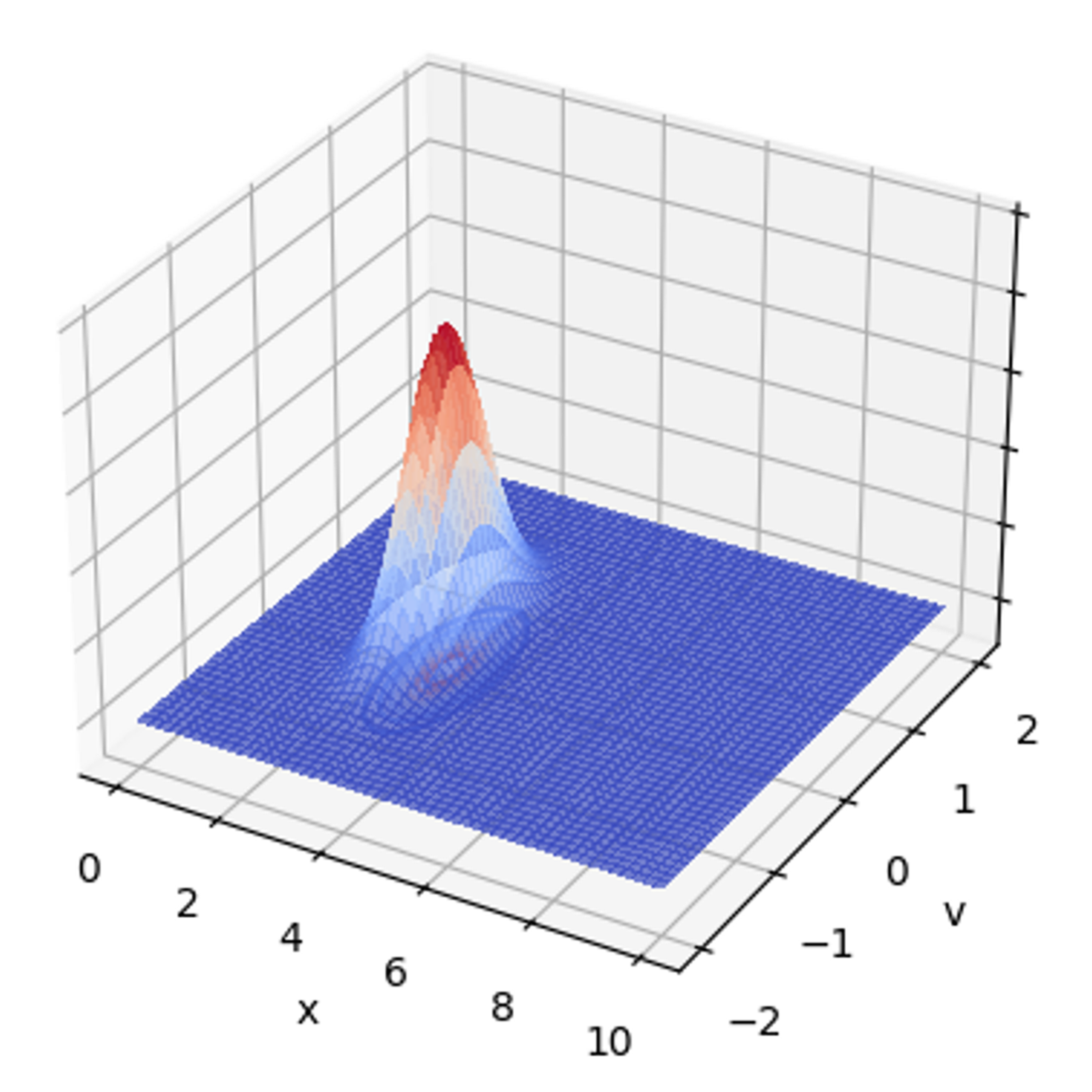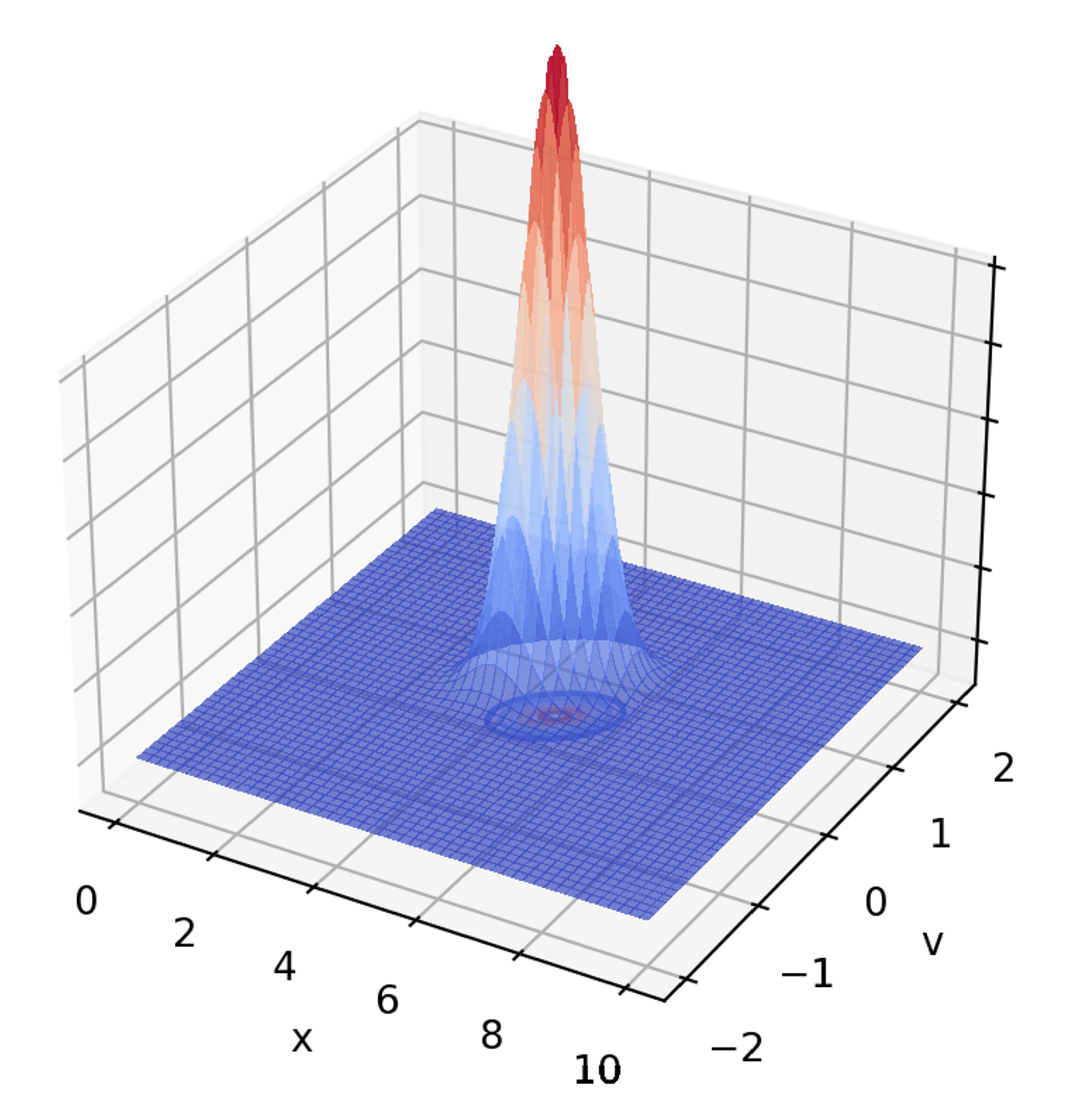If the robot receives some measurements, the probability distribution undergoes a significant correction. Each measurement provides additional information that helps refine the estimates of the robot's state, reducing uncertainty and compensating for the previous skewing and squeezing effects. The corrected probability Gaussian is depicted in Figure~\ref{fig:meas_correction}. \begin{figure}[H] \centering \includegraphics[width=0.32\textwidth]{imgs/squeezing_end.png} \caption{Probability after the measurement step.} \label{fig:meas_correction} \end{figure}\]

Conclusion

The Kalman Filter is a fundamental tool in control systems and signal processing, efficiently estimating states in linear systems with Gaussian noise. Its recursive structure is well-suited for real-time applications in various fields like navigation and tracking. However, the effectiveness of the Kalman Filter is constrained by its assumption that both system dynamics and measurement functions are linear. This limitation restricts its applicability to linear systems, as it struggles to accurately address deviations arising from non-linear behaviors in real-world scenarios. To manage non-linearities, adaptations such as the Extended Kalman Filter or alternative approaches like the Particle Filter are commonly employed.

Extended Kalman Filter

The Extended Kalman Filter (EKF) is an adaptation of the Kalman Filter for non-linear systems. While the Kalman Filter is restricted to linear models, the EKF allows for a broader range of applications by linearizing about the current estimate.

Non-Linear System with Gaussian Noise

The state and measurement models for a non-linear system can be expressed as: $$ \begin{align} \mathbf{x}t &= \mathbf{g}(\mathbf{x}{t-1}, \mathbf{u}_t) + \mathbf{w}
\mathbf{z}_t &= \mathbf{h}(\mathbf{x}_t) + \mathbf{v} \end{align} where $\mathbf{g}$ and $\mathbf{h}$ are non-linear functions of the state and control inputs, and ( \mathbf{w} \sim \mathcal{N}(0, \mathbf{R}_t) ) and ( \mathbf{v} \sim \mathcal{N}(0, \mathbf{Q}_t) ) represent the transition and measurement noise with covariance matrices ( \mathbf{R}_t ) and ( \mathbf{Q}_t ), respectively.

In the following picture we can see p $$

Linearization

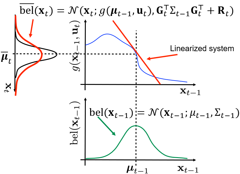
The EKF approximates these non-linear functions using the first-order Taylor expansion around the current estimate:

\[% Approximation of the non-linear state transition function \begin{equation} \mathbf{g}(\mathbf{u}_t, \mathbf{x}_{t-1}) \approx \mathbf{g}(\mathbf{u}_t, \boldsymbol{\mu}_{t-1}) + \mathbf{G}_t(\mathbf{x}_{t-1} - \boldsymbol{\mu}_{t-1}) \label{ekf-approx} \end{equation} % Approximation of the non-linear measurement function \begin{equation} \mathbf{h}(\mathbf{x}_t) \approx \mathbf{h}(\boldsymbol{\mu}_t) + \mathbf{H}_t(\mathbf{x}_t - \boldsymbol{\mu}_t), \label{ekf-measurement-approx} \end{equation} where $\mathbf{G}_t$ and $\mathbf{H}_t$ are defined as follows: % Definition of the Jacobian matrix of the state transition function \begin{equation} \mathbf{G}_t = \frac{\partial \mathbf{g}(\mathbf{x} = \boldsymbol{\mu}_{t-1}, \mathbf{u} = \mathbf{u}_t)}{\partial \mathbf{x}} \label{jacobian-matrix} \end{equation} % Definition of the Jacobian matrix of the measurement function \begin{equation} \mathbf{H}_t = \frac{\partial \mathbf{h}(\mathbf{x} = \boldsymbol{\mu}_t)}{\partial \mathbf{x}} \label{jacobian-measurement-matrix} \end{equation} The state-transition and measurement probabilities are modeled as follows: % State-transition probability for non-linear system \begin{equation} p(\mathbf{x}_t | \mathbf{x}_{t-1}, \mathbf{u}_t) \approx \mathcal{N}\left(\mathbf{x}_t; \mathbf{g}(\boldsymbol{\mu}_{t-1}, \mathbf{u}_t) + \mathbf{G}_t(\mathbf{x}_{t-1} - \boldsymbol{\mu}_{t-1}), \mathbf{R}_t\right) \label{nonlin-st-pst} \end{equation} % Measurement probability for non-linear system with predicted (a priori) state estimate \begin{equation} p(\mathbf{z}_t | \mathbf{x}_t) \approx \mathcal{N}\left(\mathbf{z}_t; \mathbf{h}(\overline{\boldsymbol{\mu}}_t) + \mathbf{H}_t(\mathbf{x}_t - \overline{\boldsymbol{\mu}}_t), \mathbf{Q}_t\right) \label{nonlin-meas-pst} \end{equation} 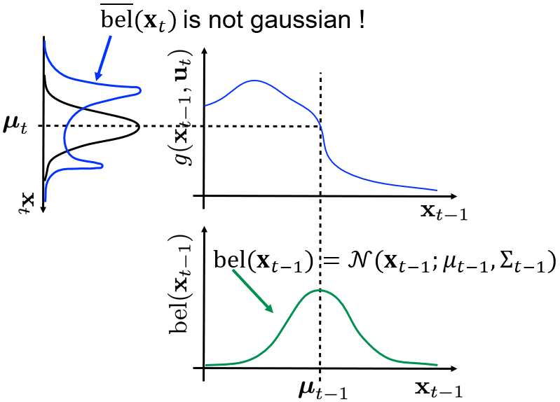In the following figures, \ref{fig:nonlinGauss} and \ref{fig:linearizedEKF}, we can observe the propagation of the prior belief, represented by the \textcolor{mygreen}{Green Gaussian}, through a non-linear system (Figure \ref{fig:nonlinGauss}) and a linearized system (Figure \ref{fig:linearizedEKF}). \begin{figure}[H] \centering \begin{minipage}[b]{0.48\textwidth} \includegraphics[width=\textwidth]{imgs/nonlin_gauss_intuition.png} \caption{Non-linear system propagation.} \label{fig:nonlinGauss} \end{minipage} \hfill \begin{minipage}[b]{0.48\textwidth} \includegraphics[width=\textwidth]{imgs/linearized_intuition_EKF.png} \caption{Linearized system propagation.} \label{fig:linearizedEKF} \end{minipage} \end{figure}\]

Implementation of Extended Kalman Filter

\[Combining the principles of the Bayes filter (equations \ref{bayes-prior} and \ref{bayes-posterior}), with prerequisities (equations \ref{st-pst} and \ref{m-pst}) and the properties of linearized Gaussian systems (equations \ref{nonlin-st-pst} and \ref{nonlin-meas-pst}), we can derive the Kalman filter update equations: \begin{itemize} \item \textbf{Prediction step} (new action \( \mathbf{u}_t \)): \begin{align} \overline{\boldsymbol{\mu}}_t &= \mathbf{g}(\boldsymbol{\mu}_{t-1}, \mathbf{u}_t) \\ \overline{\boldsymbol{\Sigma}}_t &= \mathbf{G}_t \boldsymbol{\Sigma}_{t-1} \mathbf{G}_t^\top + \mathbf{R}_t \\ \overline{\text{bel}}(\mathbf{x}_t) &= \mathcal{N}({\mathbf{x}_t};\overline{\boldsymbol{\mu}}_t, \overline{\boldsymbol{\Sigma}}_t) \end{align} \item \textbf{Measurement update} (new measurement \( \mathbf{z}_t \)): \begin{align} \mathbf{K}_t &= \overline{\boldsymbol{\Sigma}}_t \mathbf{H}_t^\top (\mathbf{H}_t \overline{\boldsymbol{\Sigma}}_t \mathbf{H}_t^\top + \mathbf{Q}_t)^{-1} \\ \boldsymbol{\mu}_t &= \overline{\boldsymbol{\mu}}_t + \mathbf{K}_t (\mathbf{z}_t - \mathbf{h}(\overline{\boldsymbol{\mu}}_t)) \\ \boldsymbol{\Sigma}_t &= (\mathbf{I} - \mathbf{K}_t \mathbf{H}_t) \overline{\boldsymbol{\Sigma}}_t \\ \text{bel}(\mathbf{x}_t) &= \mathcal{N}({\mathbf{x}_t};\boldsymbol{\mu}_t, \boldsymbol{\Sigma}_t) \end{align} \end{itemize}\]

Conclusion

The Extended Kalman Filter extends the Kalman Filter to non-linear systems by linearizing about the current state estimate. However, this approach introduces errors due to approximation, particularly when the system dynamics or measurements are highly non-linear. These errors can lead to inaccuracies and potential divergence of the filter, especially with poor initial estimates or significant non-linear deviations. Thus, for systems with strong non-linearities, more robust methods like the Unscented Kalman Filter or Particle Filter may provide better performance