Particle Filter
Particle filters are used in robotics for estimating the probability distribution of a robot’s state $p(x)$, especially useful in scenarios where processes are non-linear or involve non-Gaussian noise. The particle filter represents the unknown probability distribution $p(x)$ using a set of particles and updates these particles through prediction and correction steps based on new data.
The transition probability $p(x_t \mid x_{t−1},u_{t−1})$ describes the likelihood of the robot transitioning from one state $x_{t−1}$ to another $x_t$ given a particular action $u_{t−1}$. This could be modelled using odometry data, which might, for example, be assumed Gaussian with a known standard deviation, reflecting the inherent uncertainty in the robot’s movement.
The measurement probability $p(z \mid x_t)$ quantifies how likely it is to observe a particular measurement $z$, such as the distance from a known marker, given the robot’s current state $x_t$. The accuracy of this measurement is also modelled by a probability distribution, accounting for possible errors in sensor data.
How does the algorithm work
Let’s explore how this algorithm works with a practical example. Imagine a red blob in a simple 1D world where it can only move along the x-axis in a positive direction. The blob is somewhere in the environment shown below, but it doesn’t know its exact location. However, it can estimate its movement from one position to another through the transitional probability $p(x_t \mid x_{t−1},u_{t−1})$ and, it can detect when a door is directly in front of it, using $p(z \mid x_t)$. Let’s help the blob localize itself in this known environment!
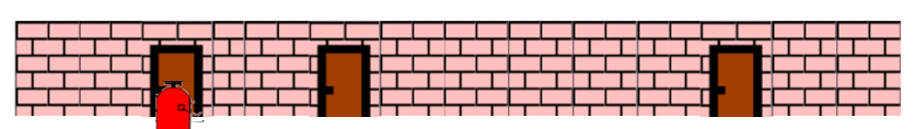 Blob in the environment.
1. Initialize particles
Since the blob has no idea where it is, and neither do we, the algorithm starts by initializing particles to represent potential positions. Given no prior information about the blob’s initial state $p(x_0)$, we will distribute $N$ particles $\mathcal{L} = \{ x_0^1, \dots, x_0^N \}$ uniformly across the entire room to positions $x_0^i$, assigning each particle an equal weight of $\frac{1}{N}$ (i for each particle). This approach reflects our complete uncertainty about the blob’s location. Utilizing a higher number of particles can provide a more precise estimation of $p(x)$, but this comes at the cost of increased computational and memory demands.
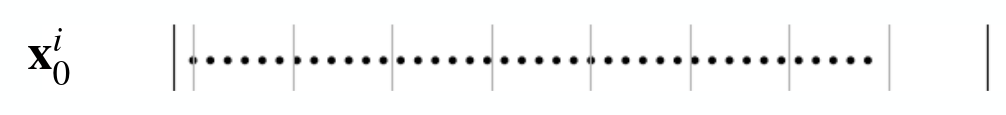 Our initial hypothesis of the blob state is uniformly distributed over the whole environment.
2. Prediction step: Blob Moved!
The blob reported moving approximately $u_{t-1} = 0.3$ meters to the right. However, given the inherent uncertainties in its reporting (since it’s only a blob), we treat this movement information cautiously. Therefore, the transitional probability $p(x_t \mid x_{t−1},u_{t−1})$ is modelled using a Gaussian distribution, reflecting the potential inaccuracies in the blob’s movement measurement. We can express this as
\[p(x_t^i \mid x_{t−1}^i,u_{t−1}^i) = \mathcal{N}(x_{t-1}^i + u_{t-1}, \sigma^2).\]We then adjust each particle’s position by sampling from $\mathcal{N}(x_{t-1}^i + u_{t-1}, \sigma^2)$, updating their estimated positions based on the blob’s reported movement.
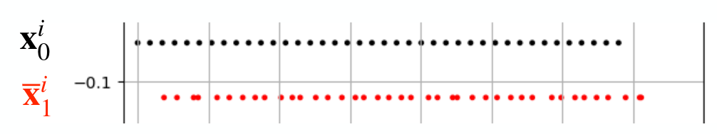 Prediction of the blob movement in red.
3. Measurement update: Blob smells the doors!
The blob can tell us if he smells the doors or not. This gives us information about the current state of the blob since the environment is known. In this step, we adjust the weights $w_t^i$ of the particles based on the measurement probability $w_t^i = p(z_t \mid x_t^i)$. This probability reflects how likely each particle’s estimated position aligns with the blob’s sensory input.
In our scenario, if the blob smells the doors, the weights for particles that are close to the known door positions are increased, reflecting a higher likelihood that these particles represent the blob’s actual position. If the blob does not smell the doors, we increase the weights of particles that are farther from the doors. This proportional adjustment ensures that each particle’s weight corresponds to the plausibility of the sensory data given the particle’s estimated location.
Additionally, the weights of all particles are normalized so that they sum up to 1, ensuring that the weights represent a valid probability distribution over the particle set.
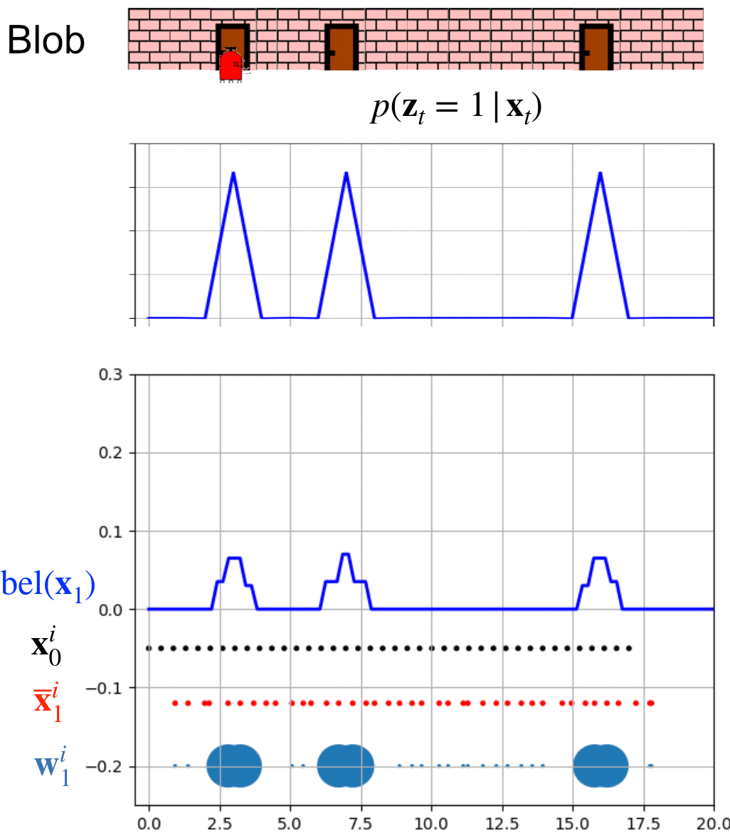
\[w^i_{\text{norm}} = \frac{w^i}{\sum_{i=1}^N w^j}\] 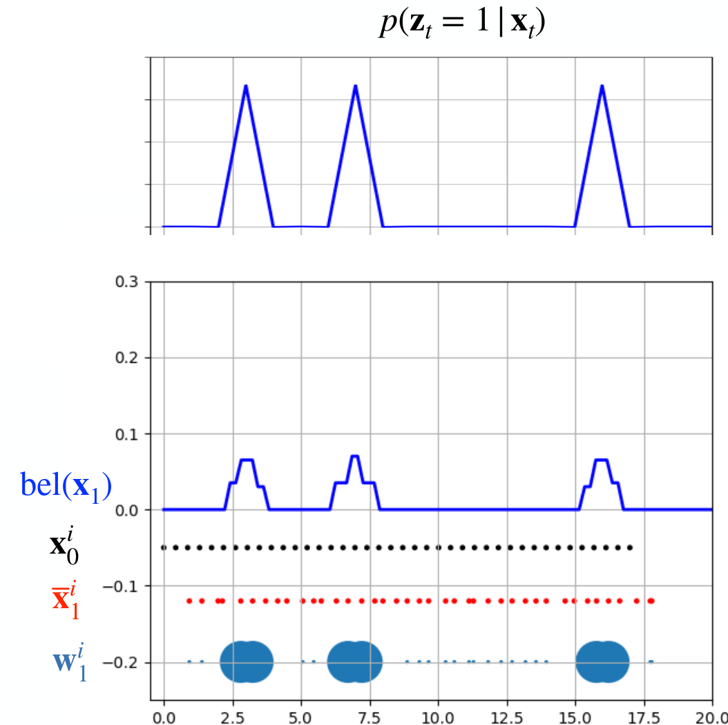 Blob detected doors at this moment, evident from the probability $p(z_t = 1 \mid x_t)$. Particles are adjusted based on this detection, with their weights reflecting the likelihood of each particle's state. Our belief about the system’s state $bel(x)$, is then updated by integrating the weights and positions of these particles. The process of $bel(x)$ reconstruction will be explained later.
4. Particle resampling.
As the particle filter gains more information, maintaining a uniform distribution of particles across the entire map becomes inefficient. To optimize our estimation of $p(x)$, the resampling process comes into play. This process systematically eliminates particles with very low weights, which represent less likely positions, and duplicates particles with very high weights. This adjustment not only focuses the computational effort on more probable states but also ensures that the density of particles is greater in areas of higher likelihood. We will deal with a detailed explanation of the resampling process later.
 Particles are resampled around positions with the highest probability. Do not be fooled by the image, the number of particles is still $N$, and some of them just share the same robot state.
5. Go back to step 2
The particle filter algorithm cycles through prediction, measurement, and resampling steps over time. Now, let’s watch the following animation to see how Blob localizes itself in the environment.
 This animation shows 8 whole iterations of the particle filter.
Why does it work?
As previously mentioned, each particle in the filter represents a hypothesis about the robot’s state within the probability distribution $p(x)$. Our belief about the robot’s state, denoted as $bel(x)$, can be reconstructed by integrating the particles. Regions, where particles are more densely aggregated, correspond to higher probability areas in our belief of the robot’s state.
Another perspective on probability density is to view each particle’s weight as an estimate of probability. The greater the weight of a particle, the greater the confidence in that particle’s state hypothesis, and hence, the higher the probability that the robot is in that state according to our belief. As we assign weights to our particles we will use the density approach.
We have a set of weighted samples, particles given as:
\[\mathcal{L} = \bigl\{ \langle x^i, w^i \rangle\bigl\}_{i = 1, \dots, N}\]These samples represent the posterior probability approximation
\[bel(x) = \sum_{i=1}^N w^i \cdot \delta_{x^i},\]where $\delta_{x^i}$ represents dirac impulse at position/state $x^i$.
Our baseline particles are sampled from our belief $bel(x)$. But in order to estimate $p(x)$ we need to generate samples from it and that is impossible. This is where the importance sampling principle comes into play. By weighting the samples from $bel(x)$ with weights proportional to the ratio of $p(x)$ to $bel(x)$, we can effectively estimate the true probability distribution $p(x)$.
\[w = \frac{p(x)}{bel(x)}\]But how do we know that weights are proportional to the ratio between $p(x)$ and $bel(x)$? The answer lies in our measurement model. This model assigns higher weights to the particles, or hypotheses, that align with our knowledge of the environment. Essentially, while we generate possible robot positions from an arbitrary probability distribution, our measurement model (for example marker detections), assigns higher weights to particles that more closely correspond to the unknown true distribution $p(x)$.
Resampling
Resampling is a process that takes the current states and weights of particles as inputs and outputs a new, resampled set of particles. The goal of resampling is to concentrate particles around the most probable states of the robot at the current iteration.
Multinomial Resampling
The idea behind this resampling method involves computing a cumulative sum of the normalized weights. This sum results in an array of values ranging from 0 to 1, with each subsequent value being greater than or equal to the previous.
To resample, a random number is generated within the range of 0 to 1. The new particle is then selected based on the interval into which this random number falls. Each interval corresponds to a particle, and the size of the interval is proportional to the particle’s normalized weight. Larger intervals correspond to particles with higher weights, thus increasing their likelihood of selection.
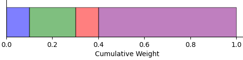
Let’s visualize the resampling process with an example. Suppose we have four particles with weights $\{0.1, 0.2, 0.1, 0.6\}$ and positions $\{1.0, 1.5, 2.0, 2.3\}$. First, we compute the cumulative sum of the normalized weights, resulting in an array of cumulative values.
We can visually represent these cumulative weights as sections of a line segment ranging from 0 to 1. The cumulative sum for our weights would split the segment into intervals: $[0, 0.1]$, $(0.1, 0.3]$, $(0.3, 0.4]$, and $(0.4, 1.0]$. Each interval represents a certain particle.
Next, we generate four random numbers within the range of 0 to 1: $\{0.74, 0.574, 0.877, 0.303\}$. Each number determines the selection of a new particle based on the interval it falls into:
- 0.74, 0.574, and 0.877 fall into the interval $(0.4, 1.0]$, corresponding to the position 2.3.
- 0.303 falls into the interval $(0.3, 0.4]$, corresponding to the position 2.0.
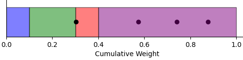
In the end, we end up with new particles at positions $\{2.3, 2.3, 2.3, 2.0\}$ with weights equal to $w^i = \frac{1}{N} = 0.25$. These new particles indicate a higher likelihood of the robot being at position 2.3, as reflected by the frequency of selection based on the random numbers generated.
Stochastic universal resampling
The Stochastic universal resampling starts similarly to multinomial resampling by computing the cumulative sum of the normalized weights. After that, the interval from $[0, 1]$ is split into $N$ equal segments and a random number $s$ is generated in range $[0, \frac{1}{N}]$. After that, $N$ numbers $t_i = s + i \cdot \frac{1}{N}$ are generated for $i \in [0,\dots,N-1]$. For each $i$, a new particle will be resampled based on the current index. The index starts at $1$ and it increments by $1$ whenever $t_i > c_{\text{index}}$, where $c$ denotes the cumulative sum array. The index is incremented till $t_i < c_{\text{index}}$. We will again visualize this resampling algorithm by an example.
We have four particles with weights $\{0.1, 0.2, 0.1, 0.6\}$ and positions $\{1.0, 1.5, 2.0, 2.3\}$. The cumulative sum is $c = \{0.1,0.3,0.4,1.0\}$. We generate random number $s = 0.02$ from interval $[0, \frac{1}{N}] = [0, \frac{1}{4}]$, leading to points $t_i = \{0.02,0.27,0.52,0.77\}$. Number $t_1 = 0.02$ is lower than $c_1 = 0.1$ therefore the index stays at $1$. The first generated particle is on position $x = 1.0$, corresponding to the first weight and first value $c_1$ in the cumulative sum. Number $t_2 = 0.27$ is again higher $c_1 = 0.1$, and lower than $c_3 = 0.4$, therefore the index is increased to $2$. The second generated particle is in position $x = 1.5$, corresponding to the second weight. The $t_3 = 0.52 > c_2 = 0.3$ and also $t_3 = 0.52 > c_3 = 0.4$,therefore the index is increased to $4$. The third and fourth particle is generated at position $x = 2.3$, corresponding to the fourth weight. Similarly, multinomial resampling all new particles share the same weight $w = 0.25 = \frac{1}{N}$.
Comparison
Multinomial resampling tends to exhibit higher variance among resampled particles and operates with a time complexity of $\mathcal{O}(N \cdot \log N)$. In contrast, Stochastic Universal Resampling (SUR) is a preferable alternative due to its linear time complexity of $\mathcal{O}(N)$ and reduced variance in the resampled particles. This makes SUR both faster and more statistically efficient.
Where does it break?
The particle filter algorithm relies on generating some particles close to the actual state of the robot. If no particles are generated near the true robot state, the algorithm may converge to an incorrect estimation of the robot’s state $p(x)$. Resampling makes this issue even worse, by potentially increasing the number of particles near an incorrect hypothesis, especially if measurements mistakenly assign higher weights to these particles. Therefore, it’s important to have enough particles near the real location of the robot to keep the algorithm working correctly.
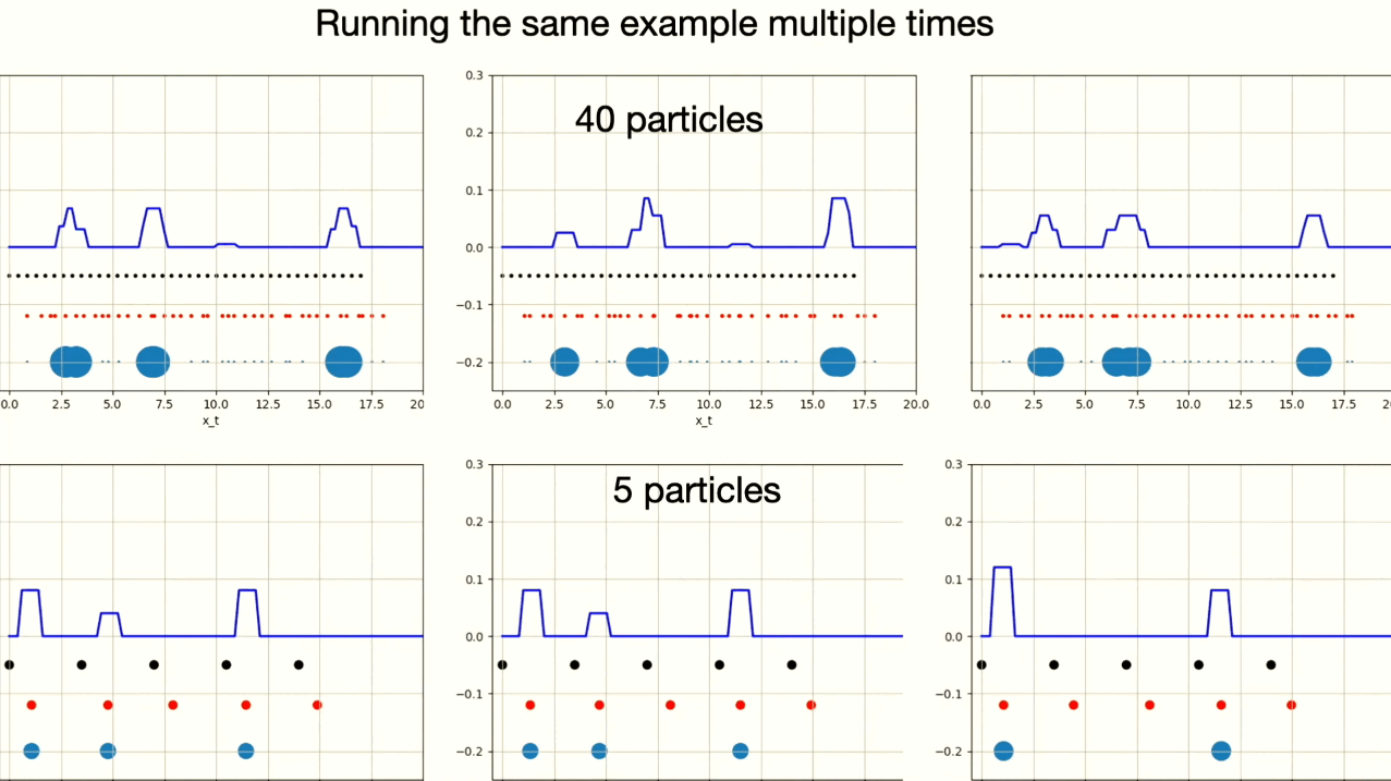
This example shows six different instances of particle filter algorithm. You can observe that one instance with 5 particles converged on the wrong robot position.
Additional materials
This video explains the particle filter itself. We highly recommend watching it, if you are still a little confused about what exactly is measurement probability. This jupyter notebook explains particle filters with code python code snippets, which may help you understand the topic better. Lastly, if you are interested in more theory behind particle filters, you can check out the Probabilistic Robotics book.
Author: Michal Kasarda