Sampling-Based Motion Planning I
These notes explain Probabilistic Roadmaps (PRM), Rapidly-Exploring Random Trees (RRT) and their optimal / informed variants.
They aim to give you all the theory you need for an exam-level understanding—without re-reading the full slide deck.
Table of contents
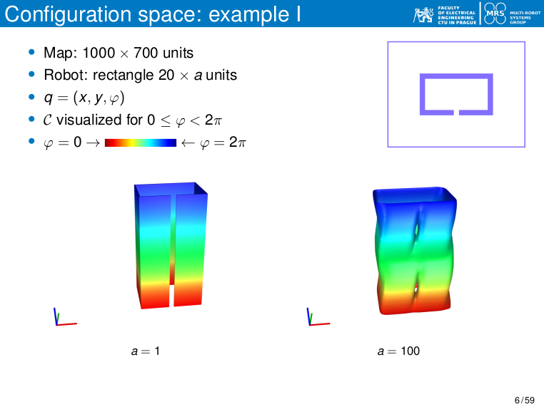
Configuration Space (C-space)
-
Definition A configuration $q$ captures every degree of freedom (DOF) of the robot.
The set of all configurations is denoted $C$ (dimension = DOFs). -
Free & obstructed regions
\(C_{\text{obs}} = \Bigl\{\,q\in C \;\Big|\; A(q)\cap O \neq \varnothing \Bigr\},\qquad C_{\text{free}} = C \setminus C_{\text{obs}}.\)Where:
- $A(q)$ is the occupied region in the workspace by the robot when it is in configuration $q$.
It accounts for the shape and size of the robot at that pose. - $O$ is the set of all obstacles in the workspace.
This can include static objects, walls, furniture, etc.
- $A(q)$ is the occupied region in the workspace by the robot when it is in configuration $q$.
-
Why this is difficult in practice
- High dimensionality → not reasonable discretization due to memory/time limits.
- Narrow passages are tiny but crucial for connectivity.
- Even simple-looking obstacles in the workspace (W) can result in very complex shapes in the configuration space (C), due to the non-trivial way the robot’s geometry $A$ interacts with the obstacles $O$.
Sampling-Based Motion Planning
Sampling-based motion planning is designed to work even when the geometry of the environment is too complex or high-dimensional to model explicitly.
Rather than building a complete map of the configuration space, we explore it by sampling and using a collision checker as a “black box”.
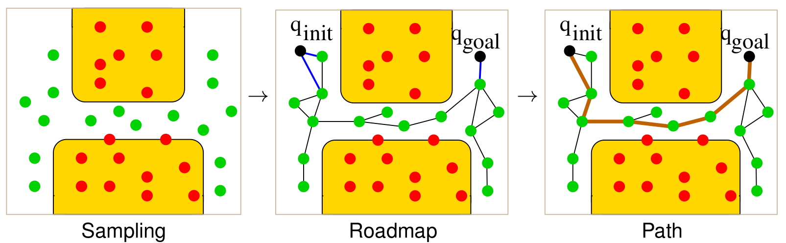
The basic pipeline involves four main steps:
Sampling the Configuration Space
We randomly sample configurations $q \in C$, where each configuration fully specifies the state of the robot (e.g., position, orientation, joint angles).
This process is done uniformly or with bias (e.g., towards goal, edges, or low-density areas) depending on the planner.
These samples may land in either:
- $C_{\text{free}}$ — the robot is in a collision-free state.
- $C_{\text{obs}}$ — the robot intersects an obstacle and the configuration is invalid.
A collision checker is used to determine this classification. It takes a robot configuration $q$ and returns whether $A(q) \cap O = \varnothing $.
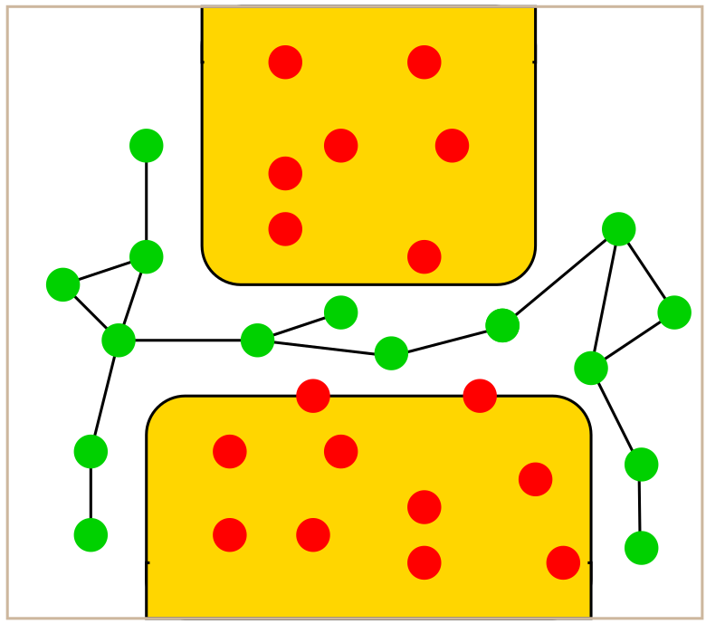
Collision Checking & Classification
Every sampled configuration is tested:
- If $q \in C_{\text{free}}$, it is accepted.
- If $q \in C_{\text{obs}}$, it is discarded.
This is what makes sampling-based methods powerful: they only require a collision-checking function, not an analytical model of the free space.
Building a Roadmap with Local Planning
Next, we attempt to connect the accepted samples using a local planner.
- For each pair of nearby nodes $q_a$ and $q_b$, we try to generate a short trajectory $\tau(t)$ that lies entirely within $C_{\text{free}}$.
- This is often done by interpolating between the two configurations and checking for collisions along the way.
Formally: \(\tau:[0,1] \rightarrow C_{\text{free}}, \qquad \tau(0) = q_a,\quad \tau(1) = q_b\)
If such a trajectory exists, we add an edge between $q_a$ and $q_b$ in the roadmap.
This graph of sampled nodes and valid edges is called the roadmap. It is an implicit representation of the accessible parts of $C_{\text{free}}$.
Path Planning on the Roadmap
Once the roadmap is constructed:
- We insert $q_{\text{init}}$ and $q_{\text{goal}}$ into the graph.
- Connect them to nearby free nodes using the local planner.
- Apply a graph search algorithm (e.g., Dijkstra or A*) to find a valid path.
The final path is a sequence of valid connections through sampled configurations that approximate a feasible solution through $C_{\text{free}}$.
Why This Works
Sampling-based planning avoids the need for an explicit map of the configuration space.
- Even in high-dimensional spaces, it can build a good approximation by focusing only on reachable, collision-free regions.
- Its success depends heavily on sampling density, connectivity, and the quality of the local planner.
These methods are probabilistically complete:
If a valid path exists, the probability that the algorithm finds it approaches 1 as the number of samples goes to infinity.
Local Planners & Their Role
| Type | Works for | Notes |
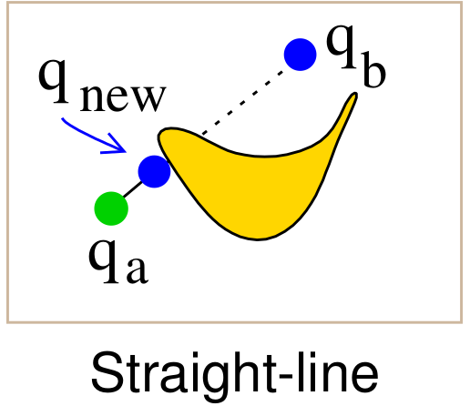
|---|---|---|
| Straight-line | Systems without kinematic/dynamic constraints | Cheapest; just interpolate and collide-check. |
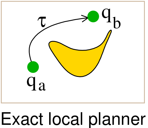
| Exact | Simple kinodynamic systems (e.g. Dubins car) | Analytic solution of the two-point BVP. |
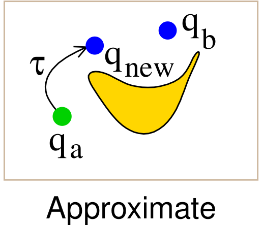
| Approximate | Any dynamics | Forward-simulate control for $\Delta t$; may fail in clutter. |
The better your local planner, the fewer samples you need — but the slower each connection test becomes.
Single-query vs Multi-query Planning
Sampling-based planners differ in how they construct and reuse planning data:
| Feature | Multi-query (e.g. PRM) | Single-query (e.g. RRT) |
|---|---|---|
| Purpose | Multiple start/goal queries | One-time planning |
| Structure | Global roadmap over $C_{\text{free}}$ | Tree grown toward goal |
| Reusability | Yes | No |
| Construction time | Higher | Faster |
| Best use case | Frequent planning, replanning | Fast planning, one-time goal |
| Example algorithms | PRM, sPRM, PRM* | RRT, RRT*, EST |
- Multi-query planners (like PRM) build a reusable roadmap and are ideal when many queries must be answered in the same space.
- Single-query planners (like RRT) focus on quickly solving one planning problem, discarding the structure afterward.
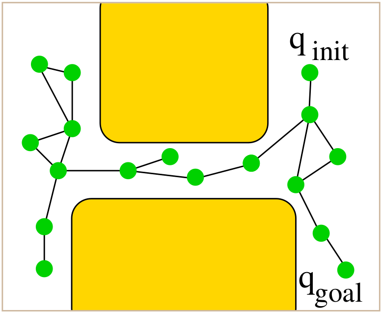
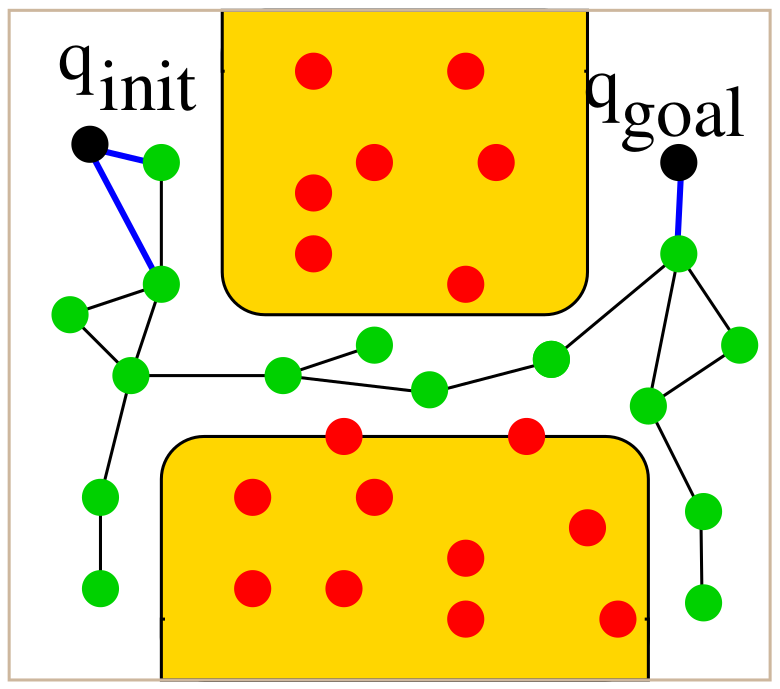
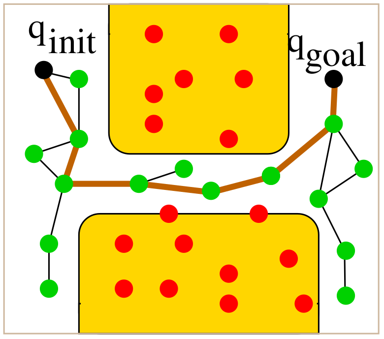
Probabilistic Roadmap (PRM)
Goal Build a reusable roadmap covering $C_{\text{free}}$; answer many start/goal queries quickly.
Construction (Learning Phase)
- Draw $n$ collision-free samples ${q_i}$.
- For every $q_i$, identify neighbours (either $k$ nearest or within radius $r$).
- Call the local planner to attempt connections; add an undirected edge if successful.
The resulting graph may contain many cycles (good for robustness).
Query Phase
- Insert $q_{\text{init}}$ and $q_{\text{goal}}$, connect them to nearby roadmap vertices, then run Dijkstra/A*.
- Because the heavy sampling work is already done, queries are fast.
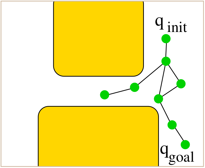
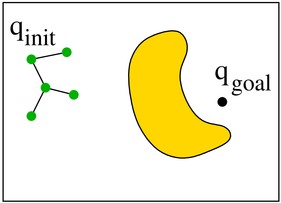
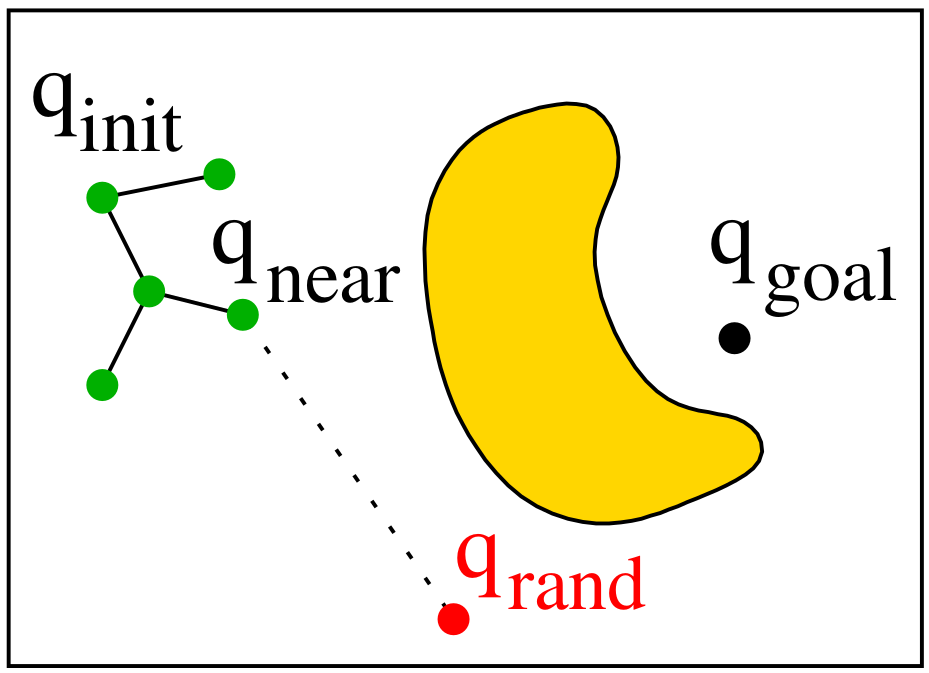
Rapidly-Exploring Random Tree (RRT)
RRT is a single-query planner that incrementally builds a tree rooted at the initial configuration $q_{\text{init}}$ and expands toward random samples.
The key idea is to bias growth toward unexplored regions of the space using random sampling and nearest-neighbor expansion.
How It Works
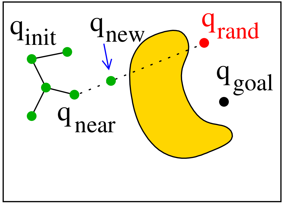
- Sample a random configuration $q_{\text{rand}}$ in $C$.
- Find the nearest tree node $q_{\text{near}}$ to $q_{\text{rand}}$.
- Use a local planner to extend from $q_{\text{near}}$ toward $q_{\text{rand}}$.
- If the motion is collision-free, add $q_{\text{new}}$ to the tree.
- Stop if $q_{\text{new}}$ is close enough to $q_{\text{goal}}$.
Key Properties
- Fast: No need to cover the whole space.
- Exploratory: Biased toward large Voronoi regions (unexplored space).
- Probabilistically complete: If a solution exists, RRT will find it eventually.
- Not optimal: The path found is often suboptimal.
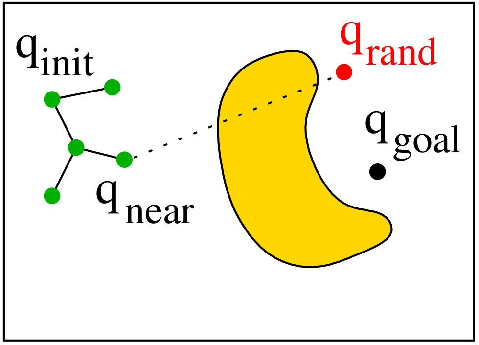
RRT Tree Expansion Variants
To grow the tree, we try to connect the nearest existing node $q_{\text{near}}$ to a random sample $q_{\text{rand}}$.
This is done by attempting a straight-line expansion between them.
There are three common strategies (variants) for how to perform this extension:
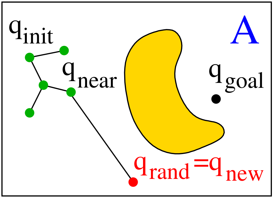
Variant A – Direct Connect
- If the segment $S = \text{line}(q_{\text{near}}, q_{\text{rand}})$ is fully collision-free, add $q_{\text{rand}}$ as a new node: \(q_{\text{new}} = q_{\text{rand}}\)
- Pros:
- Fastest growth of the tree.
- Fewer nodes needed to cover large areas.
- Cons:
- Requires checking the entire segment.
- Harder to implement with some nearest-neighbor structures.
- May fail in cluttered or narrow spaces.
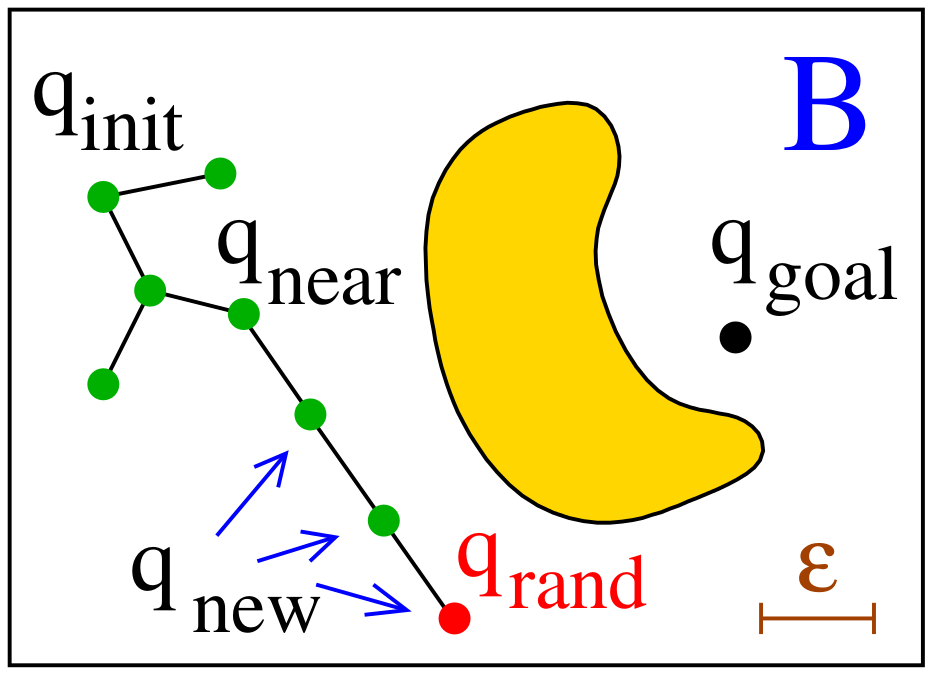
Variant B – Discretized Extension
- Discretize $S$ into small steps (e.g. every $\varepsilon$ units).
- Add all valid intermediate configurations as nodes to the tree.
-
Most commonly used in practice.
- Pros:
- Allows gradual growth through narrow regions.
- Easier to find nearest neighbors.
- Cons:
- Slightly slower than A (more collision checks).
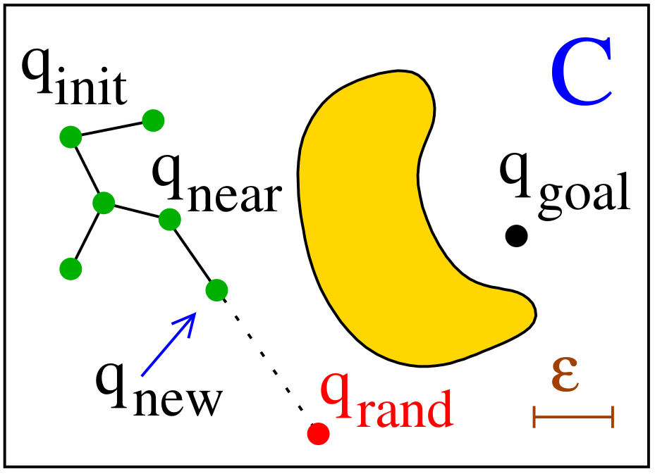
Variant C – Fixed Step Extension (Classic RRT)
- Move from $q_{\text{near}}$ a fixed step size $\varepsilon$ toward $q_{\text{rand}}$: \(q_{\text{new}} \in S \quad \text{such that} \quad \|q_{\text{new}} - q_{\text{near}}\| = \varepsilon\)
-
Add $q_{\text{new}}$ only if the motion is collision-free.
- Pros:
- Simple to implement.
- Enables fast nearest-neighbor search (uniform spacing).
- Cons:
- Slow tree growth compared to A and B.
Voronoi Bias in RRT
One of the key features that makes RRT effective is its natural Voronoi bias.
When we sample a random configuration $q_{\text{rand}}$ from the configuration space, we expand the tree from the nearest existing node $q_{\text{near}}$. But in high-dimensional space, some nodes are surrounded by more unexplored free volume than others.
Each node $q_i$ in the tree effectively “owns” a region around it — called its Voronoi region — which consists of all points in $C$ that are closer to $q_i$ than to any other node in the tree: \(\text{Vor}(q_i) = \left\{ q \in C \;\middle|\; \|q - q_i\| \leq \|q - q_j\| \;\;\forall j \ne i \right\}\)
When we draw random samples uniformly from $C$, nodes with larger Voronoi regions are more likely to be chosen for expansion, simply because there’s more “space” around them.
This creates a natural bias toward expanding the tree into unexplored areas, without any explicit planning or heuristics.
Why Voronoi Bias Matters
- Encourages exploration: The tree automatically grows toward wide-open or sparsely explored regions of $C_{\text{free}}$.
- Prevents local trapping: It avoids repeatedly sampling near already well-covered parts of the space.
- Efficient in high dimensions: Where explicit grid coverage would be infeasible.
This effect is one of the main reasons RRT works so well without needing a global roadmap or search heuristic.
Expansive-Space Tree (EST)
EST grows two trees:
-
Tree from the initial configuration:
\[\mathcal{T}_i \text{ grows from } q_{\text{init}}\] -
Tree from the goal configuration:
\[\mathcal{T}_g \text{ grows from } q_{\text{goal}}\]
Each node $q$ is assigned a weight $w(q)$ — the number of nearby nodes in the tree: \(w(q) = \left| \left\{ q' \in \mathcal{T} \;\middle|\; \|q - q'\| < r \right\} \right|\)
Nodes are selected for expansion with probability: \(P(q) \propto \frac{1}{w(q)}\)
The two trees expand until they come close, and then are connected using a local planner.
PRM* and RRT*: Making Random Planning Optimal
Both PRM* and RRT* are asymptotically optimal versions of their base algorithms.
They guarantee that the cost of the found path converges to the global optimum as the number of samples $n \to \infty$.
PRM* – Optimal Probabilistic Roadmap
PRM* improves classical PRM by carefully choosing which nodes to connect, using a connection radius that shrinks slowly with $n$:
\[r(n) = \gamma_{\text{PRM}} \left( \frac{\log n}{n} \right)^{1/d}\]Where:
- $n$ is the number of nodes,
- $d$ is the dimension of the configuration space.
This ensures:
- The roadmap becomes denser as $n$ increases,
- Every node is connected to enough neighbors to guarantee optimal paths,
- Asymptotic optimality is preserved with probabilistic completeness.
RRT* – Optimal Rapidly-Exploring Tree
RRT* improves basic RRT by choosing better parents and rewiring the tree:
-
After sampling and adding a new node $q_{\text{new}}$, choose the parent node $q_{\text{parent}}$ that minimizes:
\[\text{cost}(q_{\text{parent}}) + \text{cost}\left( \text{line}(q_{\text{parent}}, q_{\text{new}}) \right)\] -
Then, attempt to rewire nearby nodes if their path through $q_{\text{new}}$ would reduce their total cost.
The neighborhood radius also shrinks with $n$:
\[r(n) = \min \left\{ \gamma_{\text{RRT}} \left( \frac{\log n}{n} \right)^{1/d},\; \eta \right\}\]- $\eta$ is the maximum step size,
- The shrinking radius ensures optimality without losing completeness.
Summary
| Feature | PRM* | RRT* |
|---|---|---|
| Structure | Graph (roadmap) | Tree |
| Query type | Multi-query | Single-query |
| Optimality | Asymptotically optimal | Asymptotically optimal |
| Key idea | Radius-based neighbor connection | Best-parent selection + rewiring |
| Sampling goal | Dense graph in $C_{\text{free}}$ | Expand tree while optimizing cost |
Downside: Both algorithms converge slowly in practice — optimal paths appear only with many samples.
Informed & Partially Informed RRT*
Observation: A sample $q \in C$ may improve the quality of the current solution only if the combined path length from $q_{\text{init}}$ to $q$ and from $q$ to $q_{\text{goal}}$ is less than or equal to the current solution cost.
Informed RRT*
Sample only inside the prolate ellipsoid containing all points $q$ that satisfy
\(\text{dist}(q_{\text{init}},q) + \text{dist}(q,q_{\text{goal}}) \le \text{cost(current path)}.\)
Partially Informed RRT*
Shrink the sampling set further by considering ellipsoids along sub-paths—aggressive exploitation while preserving completeness.
In practice these heuristics cut runtime drastically on cluttered tasks.