How to fuse almost anything: Localization and factor graph

This chapter discusses the estimation of the robot’s position in a known environment. The first part is devoted to robot localization as a Maximum A Posteriori (MAP) estimation problem. The second part focuses on factor graph as a convenient representation of the localization problem and their use for robot position estimation.

Table of contents

Localization problem
Factor graph
1. Example of factor graph
  1. SLAM example
  2. GPS localization example
2. Lecture notes from previous year (2023/24)

Localization problem

Localization of a robot is the process of determining its position in the environment. This process uses a probability distribution and Bayes’ theorem to incrementally update the position estimate based on available measurements and the motion model.

Bayes’ theorem

Let $ A $ and $ B $ be a events and $ P(B) \neq 0 $. Then:

\[P(A \mid B) = \frac{P(B \mid A) \cdot P(A)}{P(B)}\]

where:

$ P(A \mid B) $ is the posterior probability of event $ A $ given $ B $
$ P(B \mid A) $ is the posterior probability of event $ A $ given $ B $
$ P(A) $ and $ P(B) $ are the prior probability of event $ A $ and $ B $ respectively.

In the case of localization, the equation says what is the probability that the robot is in state A given the measurement B.

Bayes’ theorem example

Let’s have a $N$ disease that 1% of the population has and a test that can detect this disease. For a sick person, the test comes out positive with a probability of 0.999 (the sensitivity of the test). In contrast, for a healthy person, the test comes out negative with a probability of 0.99 (the specificity of the test). Therefore, the test is not conclusive and the disease may not always be detected or a false alarm may occur. If a randomly selected person gives a positive test result, what is the probability that this person has the disease?

Given:

$ P(+ \mid N) = 0.999 $
$ P(- \mid \neg N) = 0.99 $
$ P(N) = 0.01 $
$ P(N \mid +) = ? $

Result:

$ P(+ \mid \neg N) = 1 - P(- \mid \neg N) = 1 - 0.99 = 0.01 $

$ P(\neg N) = 1 - P(N) = 1 - 0.01 = 0.99 $

$ P(+) = P(+ \mid N) \cdot P(N) + P(+ \mid \neg N) \cdot P(\neg N) = 0.999 \cdot 0.01 + 0.01 \cdot 0.99 \approx 0.02 $

$ $ $ P(N \mid +) = \frac{P(+ \mid N) \cdot P(N)}{P(+)} = \frac{0.999 \cdot 0.01}{0.02} \approx 0.502 $

Localization problem definition

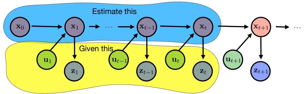
Robot localization is formally solved as a Maximum A Posteriori (MAP) estimation problem, which aims to find the most probable trajectory of the robot based on measurements and actions.

\[\mathbf{x}^* = \arg\max_x p(\mathbf{x} \mid \mathbf{z},\mathbf{u}) = \arg\max_{x_1, \dots ,x_t} p(x_0, \dots ,x_t \mid z_1, \dots ,z_t, u_1, \dots,u_t).\]

where:

$ x_0, x_1, \dots, x_t \in \mathbb{R}^n $ are true states of the robot. The state can represent, for example, temperature, position, battery voltage or robot orientation.
$ x^\ast_{0}, x^\ast_{1}, \dots, x^\ast_t \in \mathbb{R}^n$ indicates the most probable states that the robot was in based on measurements and actions
$ u_1, u_2, \dots, u_t \in \mathbb{R}^m $ are actions that lead to a change of states, i.e. $ x_t = x_{t-1} + u_t $
$ z_1, z_2, \dots, z_t \in \mathbb{R}^k $ are absolute or relative measurements to determine the state of the robot. These can be measurements from, for example, a GPS, lidar or thermometer.

Localization example: Absolute position measurements in wcf (world coordinate frame)

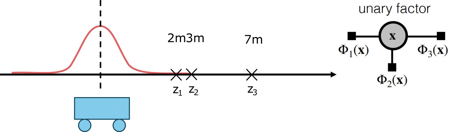
Consider a robot moving along an axis and having three absolute position measurements of 2 m, 3 m and 7 m ($z_1, z_2, z_3$). The robot can be in any state $x$ so $p(x)$ is uniform distribution. Using the MLE and Bayes’ theorem, calculate the most probable position $x^*$ of the robot based on measurements such that:

\[x^* = \arg\max_x p(x \mid z_1, z_2, z_3) = \arg\max_{x} \frac{p(z_1, z_2, z_3 \mid x) \cdot p(x)}{p(z_1, z_2, z_3)}.\]

The term $p(z_1, z_2, z_3) $ can be omitted from the calculation since it does not depend on the search position $x$ and only scales the probability. Similarly, the term $p(x) $ can be omitted since it is a uniform distribution and does not affect the function $\arg\max$. The resulting formula can also be rewritten using the logarithm:

\[x* = \arg\max_x \left( \prod_i p(z_i \mid x) \right) = \arg\min_x \sum_i -\log p(z_i \mid x).\]

The following video shows the calculation process for the discrete probability distribution $p(z \mid x) $. The robot’s position is most likely at 3 m.

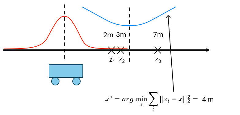
Similarly, this example can be solved for the continuous probability distribution $p(z_i \mid x)$. Specifically, for the normal distribution $ p(z_i \mid x) = \mathcal{N}(z_i;x, \sigma^2) $

\[\begin{align*} x^* &= \arg\max_x p(x \mid z_1, z_2, z_3) = \arg\max_x \left( \prod_i p(z_i \mid x) \right)= \\ &= \arg\max_x \left( \prod_i \mathcal{N}(z_i;x, \sigma^2) \right) = \arg\max_x \prod_i K \cdot \exp \left( -\frac{\|z_i-x\|_2^2}{\sigma^2} \right) = \\ &= \arg\min_x \sum_i \|z_i-x\|_2^2 = \frac{\sum_i z_i}{N}. \end{align*}\]

The following figure shows that the function takes its minimum in this example at point $4$ m.

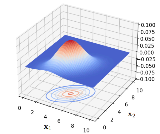
Multivariate gaussian

In case we are trying to estimate the robot’s position in space, we need to use a multivariate Gaussian probability distribution. Multivariate Gaussian is defined as follows:

\[p(x) = \mathcal{N}(x; \mu, \Sigma) = \frac{exp(-\frac{1}{2}(x-\mu)^T\Sigma^{-1}(x-\mu))}{\sqrt{(2\pi)^n\det(\Sigma)}},\]

where

$ x \in \mathcal{R}^n $ is real n-dimensional random column vector
$ \mu \in \mathcal{R}^n $ is real n-dimensional mean
$ \Sigma \in \mathcal{R}^{n \times n} $ symmetric positive definite covariance matrix.

Logarithm of Gaussian is quadratic form:

\[\log(\mathcal{N}(x;\mu, \Sigma)) = -\frac{1}{2}(x-\mu)^T\Sigma^{-1}(x-\mu) + C.\]

Localization example: Relative position measurements in rcf (robot coordinate frame)

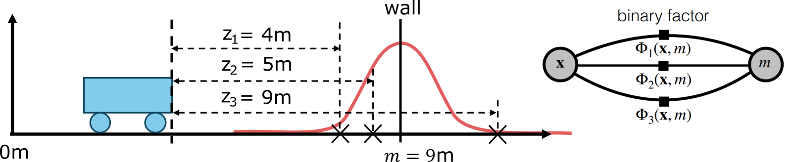
In this case, the relative position of the robot is, for example, the distance from an obstacle or marker whose position we know. The solution will be similar to the previous example, except that here we convert the position of the wall into robot coordinate system ($m-x$) and use it as a parameter of the normal distribution of measurements $p(z_i \mid x, m)= \mathcal{N}(z_i;m-x, \sigma^2)$. The calculation then looks like this:

\[\begin{align*} x^* &= \arg\max_x p(x \mid z_1, z_2, z_3, m) = \arg\max_x \left( \prod_i p(z_i \mid x,m) \right) = \\ &= \arg\max_x \left( \prod_i \mathcal{N}(z_i;m-x, \sigma^2) \right) = \arg\max_x \prod_i K \cdot \exp \left( -\frac{\|(m-x)-z_i\|_2^2}{\sigma^2} \right) = \\ &=\arg\min_x \sum_i \|m-z_i-x\|_2^2 = \frac{\sum_i m-z_i}{N}. \end{align*}\]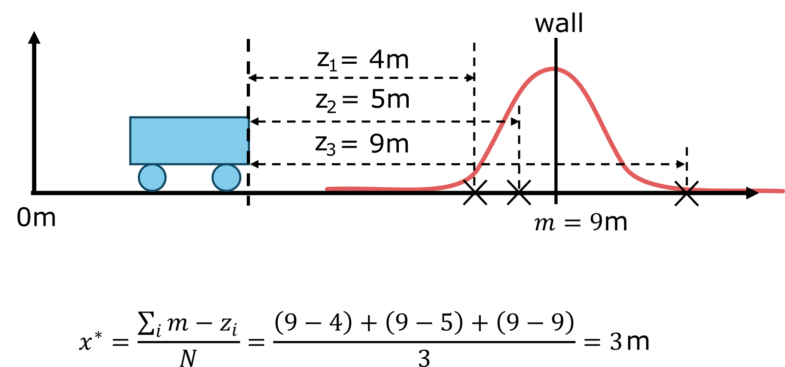

SLAM example: Realtive position measurment in rcf

In case we do not know the position of the robot or the position of the object to which we are measuring the relative position of the robot, we minimize the previous equation through two variables $x$ and $m$.

\[\begin{align*} x^* &= \arg\max_{x,m} p(x,m \mid z_1, z_2, z_3) = \arg\max_{x,m} \left( \prod_i p(z_i \mid x,m) \right) = \\ &= \arg\max_{x,m} \left( \prod_i \mathcal{N}(z_i;m-x, \sigma^2) \right) = \arg\max_{x,m} \prod_i K \cdot \exp \left( -\frac{\|(m-x)-z_i\|_2^2}{\sigma^2} \right) = \\ &= \arg\min_{x,m} \sum_i \|m-z_i-x\|_2^2 = \frac{\sum_i m-z_i}{N}. \end{align*}\]

One possible solution is $(x, m)$ = $(3, 9)$ solution from the previous example. Other solutions are all combinations of robot and wall positions that differ by $6$ m, so for example $(1, 7), (2, 8), (4, 10), \dots $ For one unique solution, we need to have, for example, at least one additional absolute solution.

Moving robot

So if we have two absolute measurements $z_1$ and $z_2$ these measurements are taken at time $t = 1$ and $t = 2$. At time $t = 1$ the robot is in state $x_1$ and we take measurment $z_1$ and at time $t = 2$ the robot is in state $x_2$ and we take measurment $z_2$. So we are trying to estimate the robot’s trajectory. This gives us two normal distributions, one for each position $x$. However, since there is a connection between the robot’s positions in time for example the constraints on its velocity we add a relative measure $ z_{12} $ of the distance $x_2-x_1$. Thus, the following computation tries to estimate $x_1$, $x_2$ and $x_2-x_1$ so as to maximize the probability of measuring $z_1$, $z_2$ and $z_{12}$ of the normal distribution belonging to a given state.

\[\begin{align*} p(z_1 \mid x_1) &= \mathcal{N}(z_1; x_1, \sigma^2)\\ p(z_2 \mid x_2) &= \mathcal{N}(z_2; x_2, \sigma^2)\\ p(z_{12} \mid x_1, x_2) &= \mathcal{N}(z_{12}; x_2-x_1, \sigma^2)\\ \end{align*}\] \[\begin{align*} (x_1^*, x_2^*) &= \arg\max_{x_1,x_2} p(x_1, x_2 \mid z_1, z_2, z_{12}) = \arg\max_{x_1,x_2} p(z_1 \mid x_1) \cdot p(z_2 \mid x_2) \cdot p(z_{12} \mid x_1, x_2)= \\ &=\arg\min_{x_1,x_2} ((z_1 - x_1)^2 +(z_2 - x_2)^2 + (z_{12} - (x_2-x_1))^2) = (1.5, 3.5) \end{align*}\]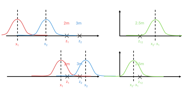

Specifically, for the figure above, we try to maximize the probability of measuring $z_1$, $z_2$ and $z_{12}$ by the normal distribution of the corresponding color. Thus, the optimal solution is in the situation where $(z_1-x_1) = (z_2-x_2) = (z_{12} -(x_2 - x_1)) = 0.5$.

Since we know that the robot should have performed the action/movement $u_2$ to reach the state $x_2$ from the state $x_1$, we can use this information in estimating its position. Using the motion probability $p(x_2 \mid x_1, u_2) = \mathcal{N}(x_2;x_1+u_2, \sigma^2)$, which expresses that if the robot was in state $x_1$ and is supposed to perform the motion action $u_2$, then in time $t=2$ it will be around state $x_2$ with normal distribution probability. Using $u_2 = 2.5$ as the action and thus supporting the relative measurement $z_{12}$, the optimal solution will not change much from the previous one. The calculation with motion propability looks as follows:

\[\begin{align*} (x_1^*, x_2^*) &= \arg\max_{x_1,x_2} p(x_1, x_2 \mid z_1, z_2, z_{12}, u_2) = \\ &= \arg\max_{x_1,x_2} p(z_1 \mid x_1) \cdot p(z_2 \mid x_2) \cdot p(z_{12} \mid x_1, x_2) \cdot p(x_2 \mid x_1, u_2) = \\ &=\arg\min_{x_1,x_2} ((z_1 - x_1)^2 +(z_2 - x_2)^2 + (z_{12} - (x_2-x_1))^2) + (x_2 -(x_1 + u_2))^2 \\ &\approx (1.4, 3.6). \end{align*}\]

Linear model and non- linear model for moving robot

If we include, for example, rotation in the robot’s motion, a non-linear trajectory is created. In the case of non-linear motion, we use the non-linear functions $h()$ and $g()$ to describe the probability model.

	Linear model	Non-linear model
Absolute measurement probability	$p(z_1 \mid x_1) = \mathcal{N}(z_1;x_1, \sigma_1^2)$	$p(z_1 \mid x_1) = \mathcal{N}(z_1;h(x_1), \sigma_1^2)$
Absolute measurement probability	$p(z_2 \mid x_2) = \mathcal{N}(z_2;x_2, \sigma_2^2)$	$p(z_2 \mid x_2) = \mathcal{N}(z_2;h(x_2), \sigma_2^2)$
Relative measurement probability	$p(z_{12} \mid x_1, x_2) = \mathcal{N}(z_{12};x_2-x_1, \sigma_{12}^2)$	$p(z_{12} \mid x_1, x_2) = \mathcal{N}(z_{12};h(x_1, x_2), \sigma_{12}^2)$
Motion probability	$p(x_2 \mid x_1, u_2) = \mathcal{N}(x_2;x_1+u_2, \sigma^2)$	$p(x_2 \mid x_1, u_2) = \mathcal{N}(x_2;g(x_1, u_2), \sigma^2)$

Factor graph

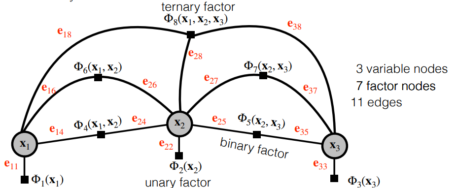
Factor graph is bipartite graph $\mathcal{G} = \lbrace \mathcal{U},\mathcal{V},\mathcal{E} \rbrace$ with two types of nodes: factors $\Phi_i \in \mathcal{U}$ and variables $x_j \in \mathcal{V}$.

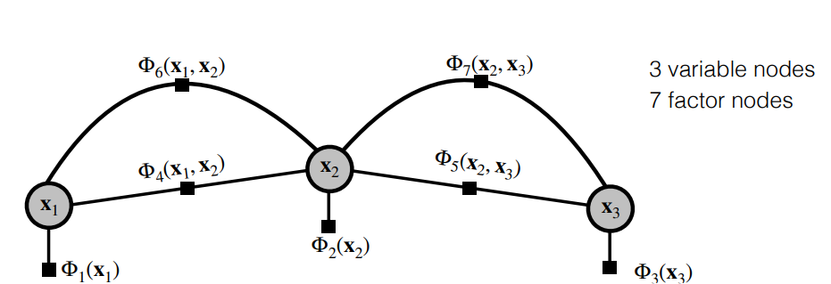
Edges $e_{ij} \in \mathcal{E}$ are always between factor nodes and variable nodes. Depending on the number of nodes with which the factor is associated it is called unary, binary, ternary, $\dots$

Factor graph is convenient visualization of (sparse) problem structure allows to simply formulate the MAP estimate in negative logarithmic space.

\[\begin{align*} x_0^*,\dots ,x_t^* = \arg\max_{x_0, \dots ,x_t} \prod_i \Phi_i(X_i) = \arg\min_{x_0, \dots ,x_t} \sum_i -log(\Phi_i(X_i)) \end{align*}\]

If factors are linear there are closed-form solution available like least square or Kalman filtr method.

Example of factor graph

SLAM example

An example with three relative measurements of the robot’s distance from an obstacle with unknown robot and wall positions can be drawn as a factor graph with two nodes (robot position and wall position) and three factors representing the three measurements depending on both robot position and wall position. The factors are binary since they depend on two parameters.

GPS localization example

The localization of the robot based on three absolute measurements of its position can be represented by a factor graph with one node (robot position) and three unary factors corresponding to the three measurements.