Sampling-Based Motion Planning II
This page provides an explanation of how to impose constraints—kinematic, dynamic, and task-related—on path planning using the algorithms introduced in previous lectures. In particular, we will focus on how to extend RRT to account for such constraints. We will also explore how to use RRT for robotic manipulators and, finally, describe the performance analysis of a general planning algorithm.
Table of contents
- Transition Equation, Forward Motion model, State Trajectory
- Motion Planning Under Differential Constraints
- Constraints - Overview
- Basic Kinematic Motion Models
- RRT + Differential Constraints
- Local Planner - Dubins Curves
- Motion Planning for Robotic Manipulators
- Performance Measurement in Motion Planning
- Planner Analysis
Transition Equation, Forward Motion model, State Trajectory
Transition Equation
We assume a transition equation of the form:
\[\dot{x} = f(x, u)\]where:
- $ x \in \mathcal{X} $ is the state vector.
- $ u \in \mathcal{U} $ is the action vector from the action space $\mathcal{U}$.
- $ \mathcal{X} $ is the state space, which may be equal to the configuration space $ \mathcal{C} $, or a phase space if dynamics are considered.
- If dynamics are included, the phase space is derived from $ \mathcal{C} $.
- Similar to configuration space, the state space $ \mathcal{X}$ can be divided into:
- $ \mathcal{X}_{\text{free}} $: free state space.
- $ \mathcal{X}_{\text{obs}} $: obstacle state space.
Forward Motion Model
- The function $f(x, u)$ is also known as the forward motion model.
State Trajectory
- Let $ \tilde{u} : [0, \infty) \to \mathcal{U} $ denote the action trajectory.
- At each time ( t ), the applied action is $ \tilde{u}(t) \in \mathcal{U} $.
- The corresponding state trajectory is given by:
where $ x(0) $ is the initial state at time $ t = 0 $.
Motion Planning Under Differential Constraints
The task is to compute an action trajectory:
\[\tilde{u} : [0, \infty) \rightarrow \mathcal{U}\]such that the resulting state trajectory $x(t)$ satisfies the following conditions:
-
Initial state: \(x(0) = x_{\text{init}}\)
-
Reaches the goal state for some $t > 0$: \(x(t) = x_{\text{goal}}\)
-
The state must always lie in the free space: \(x(t) \in \mathcal{X}_{\text{free}}, \quad \forall t\)
-
The state trajectory is defined by: \(x(t) = x(0) + \int_0^t f(x(t'), \tilde{u}(t')) \, dt'\)
Optionally:
- The state must satisfy task-specific constraints for all $t$: \(f_c(x(t)) = 0\)
Constraints - Overview
Differential constraints limit how a robot can move and are typically categorized into three types:
Kinematic Constraints
- Describe how the robot can move based on its structure.
- Given by the motion model: \(\dot{x} = f(x, u)\)
Dynamic Constraints
- Limit physical properties like speed or acceleration.
- Example: a joint must not exceed maximum velocity.
Task Constraints
- Enforced by task requirements.
- Example: end-effector must stay at a fixed distance or angle during operation.
Basic Kinematic Motion Models
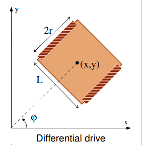
Differential Drive
- Inputs: Left and right wheel speeds ($u_l$, $u_r$)
-
Equations:
\[\begin{align} \dot{x} &= \frac{r}{2}(u_l + u_r)\cos \varphi \\ \dot{y} &= \frac{r}{2}(u_l + u_r)\sin \varphi \\ \dot{\varphi} &= \frac{r}{L}(u_r - u_l) \end{align}\]
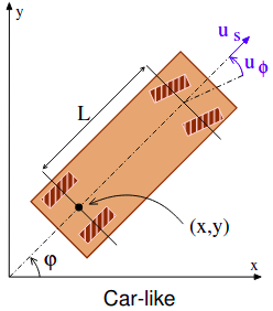
Car-like Robot
- Inputs: Forward speed ($u_s$) and steering angle ($u_\varphi$)
-
Equations:
\[\begin{align} \dot{x} &= u_s \cos \varphi\\ \dot{y} &= u_s \sin \varphi\\ \dot{\varphi} &= \frac{u_s}{L} \tan u_\varphi \end{align}\]
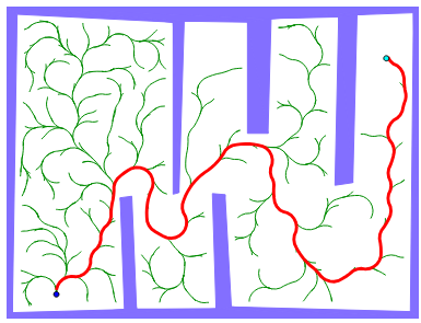
RRT + Differential Constraints
Classic RRT can be extended to handle differential constraints by using the forward motion model and a discretized input set $\mathcal{U}$.
The main idea is as follows:
- Sample a random state vector from the state space $\mathcal{X}$.
- Find the nearest neighbor to this sample in the existing tree $\mathcal{T}$.
- Integrate the motion model from the nearest neighbor over a fixed time interval $\Delta t$, using all inputs from the discretized set $\mathcal{U}$.
- This produces a set of reachable state vectors.
- Select the state with the smallest distance to the sampled state.
- Expand the tree $\mathcal{T}$ by connecting it to this new state.
This process ensures that the expansion respects the system’s dynamics and constraints.
1  Initialize tree T with x_init
2  for i = 1 to I_max do
3      x_rand ← random sample from 𝓧
4      x_near ← nearest node in T to x_rand
5      best ← ∞
6      x_new ← ∅
7      for each u ∈ 𝓤 do
8          x ← integrate f(x, u) from x_near over time Δt
9          if x is feasible and collision-free and ρ(x, x_rand) < best then
10             x_new ← x
11             best ← ρ(x, x_rand)
12     if x_new ≠ ∅ then
13         T.addNode(x_new)
14         T.addEdge(x_near, x_new)
15         if ρ(x_new, x_goal) < d_goal then
16             return path from x_init to x_goal
Local Planner - Dubins Curves
A natural question arises:
Is it always possible to connect the current tree node to a randomly sampled state?
The answer is: not always — due to differential constraints.
However, for a car-like robot moving at a constant speed $u_s = 1$, it is possible using so-called Dubins curves.
The motion model for such a system is:
\[\dot{x} = \cos \varphi \\ \dot{y} = \sin \varphi \\ \dot{\varphi} = u\]- Control input $u$ represents turning, where:
$u \in [-\tan \varphi_{\text{max}}, \tan \varphi_{\text{max}}]$
Dubins Curves
- A set of six optimal paths to connect two configurations:
LSL, LSR, RSL, RSR, LRL, RLR- L = left turn
- R = right turn
- S = straight segment
-
Dubins curves provide an exact and optimal local planner for this model.
- Any two configurations can be connected using one of these curves.
Motion Planning for Robotic Manipulators
In general, there are three ways of planning for robotic manipulators: planning in workspace and planning in joint space.
- Workspace / Cartesian / Operational Space
- The path is planned for the end-effector in workspace $\mathcal{W}$.
- Inverse Kinematics (IK) is used to compute joint configurations.
- Collision detection is done at the joint configurations.
- Potential issue: IK may fail or return multiple solutions (especially near singularities).
- Joint-Space (Configuration Space)
- The path is planned directly in joint space $\mathcal{C}$ using joint angles $q$.
- No IK is involved.
- Collision detection is performed at the planned joint configurations.
- More robust and avoids IK-related issues.
- Planning with Task-Space Bias
- Combines workspace planning and joint-space planning.
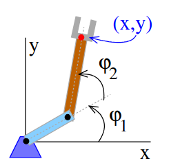
Configuration and Kinematics
- $q = (\varphi_1, \ldots, \varphi_n)$: joint configuration (for $n$ joints)
-
$x$: position (and optionally rotation) of the link or end-effector
-
Forward Kinematics:
\(x = \text{FK}(q)\) - Inverse Kinematics:
\(q = \text{IK}(x)\)- Note: IK may have singularities: Small changes in the end-effector’s position may require large joint movements
Collision Detection
- Collision checks are done in joint space, using $q$
- Let $A_i(q)$ be the position of link $i$ at configuration $q$
-
Collision detection involves checking: \(A_i(q) \cap \mathcal{O} \neq \emptyset\) where $\mathcal{O}$ represents obstacles
- For a desired end-effector pose $x$:
- Compute $q = \text{IK}(x)$
- Derive $A_i(q)$
- Check for collisions
Planning in Workspace
- Overview
- Path is planned for the end-effector in the workspace $\mathcal{W}$.
- This is a naïve application of RRT to manipulators.
- RRT Steps in Workspace
- Sample a random point $x_{\text{rand}} \in \mathcal{W}$ (i.e., end-effector position).
- Find $x_{\text{near}}$, the closest node in the tree.
- Draw a straight line from $x_{\text{near}}$ to $x_{\text{rand}}$ with resolution $\varepsilon$.
- For each intermediate waypoint $x$ on the line:
- Compute joint configuration: $q = \text{IK}(x)$
- Check for collisions at $q$
- Problems
- Singularities:
- The straight-line path in workspace may pass through a singularity.
- This can lead to unwanted or abrupt reconfigurations of the manipulator.
- Inverse Kinematics:
- Requires fast and reliable IK at each step.
- Constraints:
- Evaluating task or dynamic constraints is difficult in workspace planning.
- Singularities:
Planning in Joint Space
- Overview
- Path is planned directly in the joint space $\mathcal{C}$.
- RRT operations (sampling, tree expansion, nearest-neighbor search) are done in joint space.
- RRT Steps in Joint Space
- Define a set of allowed joint changes $\mathcal{U}$, e.g.: \(\mathcal{U} = \{ (-\Delta_1, 0), (\Delta_1, 0), (0, -\Delta_2), (0, \Delta_2), \ldots \}\)
- Sample a random configuration $q_{\text{rand}} \in \mathcal{C}$.
- Find the nearest neighbor $q_{\text{near}}$ in the tree.
- For each control input $u \in \mathcal{U}$:
- Compute $q’ = q_{\text{near}} + u$
- Check for collisions at $q’$ using $A_i(q’)$
- Add to the tree the collision-free $q’$ that minimizes distance to $q_{\text{rand}}$.
- Advantages
- No issues with singularities
- Task and dynamic constraints can be evaluated directly in joint space
- Potential Issue
- The goal state must be defined in joint space $\mathcal{C}$
Planning with Task-Space Bias
- Overview
- Combines workspace sampling with joint-space planning.
- Sampling is done in task space $\mathcal{W}$, while tree expansion happens in joint space $\mathcal{C}$.
- Each tree node stores both:
- $q \in \mathcal{C}$ (joint configuration)
- $x = \text{FK}(q) \in \mathcal{W}$ (end-effector pose)
- RRT Procedure
- Sample $x_{\text{rand}} \in \mathcal{W}$ (task space)
- Find nearest node in the tree (based on distance in $\mathcal{W}$): $x_{\text{near}}$
- Compute joint angles:
- $q_{\text{rand}} = \text{IK}(x_{\text{rand}})$
- $q_{\text{near}} = \text{IK}(x_{\text{near}})$
- Expand in joint space from $q_{\text{near}}$ toward $q_{\text{rand}}$ (e.g., in a straight line)
- If $q_{\text{new}}$ is collision-free, add:
- $q_{\text{new}}$ and $x_{\text{new}} = \text{FK}(q_{\text{new}})$ to the tree
- Advantages
- No problems with singularities
- Can evaluate task and dynamic constraints
- Goal can be specified in task space only
Performance Measurement in Motion Planning
Which Planner Is the Best?
- There are many planners, modifications, and parameters.
- No Free Lunch Theorem: No single planner works best for every problem.
- The best planner depends on the specific problem instance.
- You cannot rely solely on literature or online recommendations.
- Time complexity analysis is often not enough — you must test performance yourself.
Typical Performance Indicators
- Path quality: length, travel time, smoothness
- Runtime and memory usage
- For randomized planners:
- Statistical performance
- Success rate curve over time or trials
Good Practice
- Make your testing setup match the real-world use case as closely as possible.
- Don’t blindly trust test routines — always verify their correctness!
Planner Analysis
There are two common approaches to analyzing the performance of motion planning algorithms:
- Time Complexity Analysis
- Cumulative Probability Analysis
Time Complexity Analysis
The two most time-consuming operations in sampling-based planners like RRT are:
- Collision Detection
- Performed multiple times per iteration
- Depends on the number of geometry primitives.
- Nearest Neighbor Search
- Required to find the closest tree node to the sampled state
Time Complexity of One RRT Iteration:
-
General form: \(O(\text{nearest_neighbor} + \text{collision_detection})\)
- Assuming:
- KD-tree for nearest-neighbor search
- Hierarchical collision detection
- The complexity becomes: \(O(\log n + k \log(m_A + m_W))\)
Where:
- $n$: number of nodes in the tree
- $k$: number of collision checks
- $m_A$: number of geometric primitives in the robot (A)
- $m_W$: number of geometric primitives in the workspace (W)
Cumulative Probability
- Based on the cumulative distribution function $F(x)$
- $x$ typically represents:
- Number of iterations, or
- Runtime
- $F(x)$ gives the probability that a solution is found in less than $x$ iterations (or time)
- Applies to randomized planners only (e.g., RRT, PRM)
- Useful to compare planner performance statistically
- Shows how quickly and reliably a planner finds a solution
- Only valid for the tested scenario — results are instance-specific
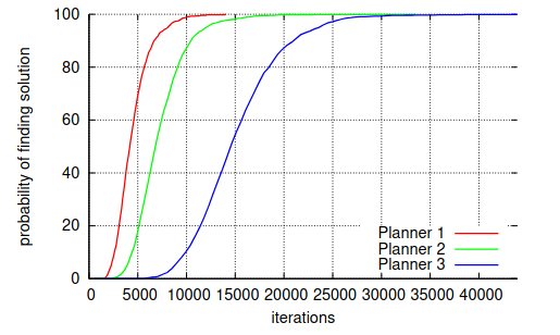
- Based on this plot, Planner 1 is statistically the best among the three for the given instance, as it reaches a higher success rate more quickly.
- Many authors present the RRT algorithm such that the randomly sampled configuration $q_{\text{rand}}$ must lie in the free space $\mathcal{C}_{\text{free}}$.
- However, from a statistical perspective, this restriction is unnecessary and even counterproductive.
- It is generally better not to impose this constraint — sampling from the entire configuration space $\mathcal{C}$ allows for better exploration and improves the chances of finding a valid connection through collision checking.