Robust loss functions
The Iterative Closest Point (ICP) algorithm is pivotal in the field of robotics for the accurate association of inliers from map and sensor point clouds within the Simultaneous Localization and Mapping (SLAM) framework. To ensure precise point matching, the operation of ICP is often conducted at high frequencies. Typically, local features are utilized in the matching process, where, in its simplest form, each point from the map is associated with the nearest point within the sensor point cloud.
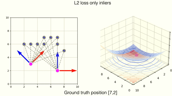
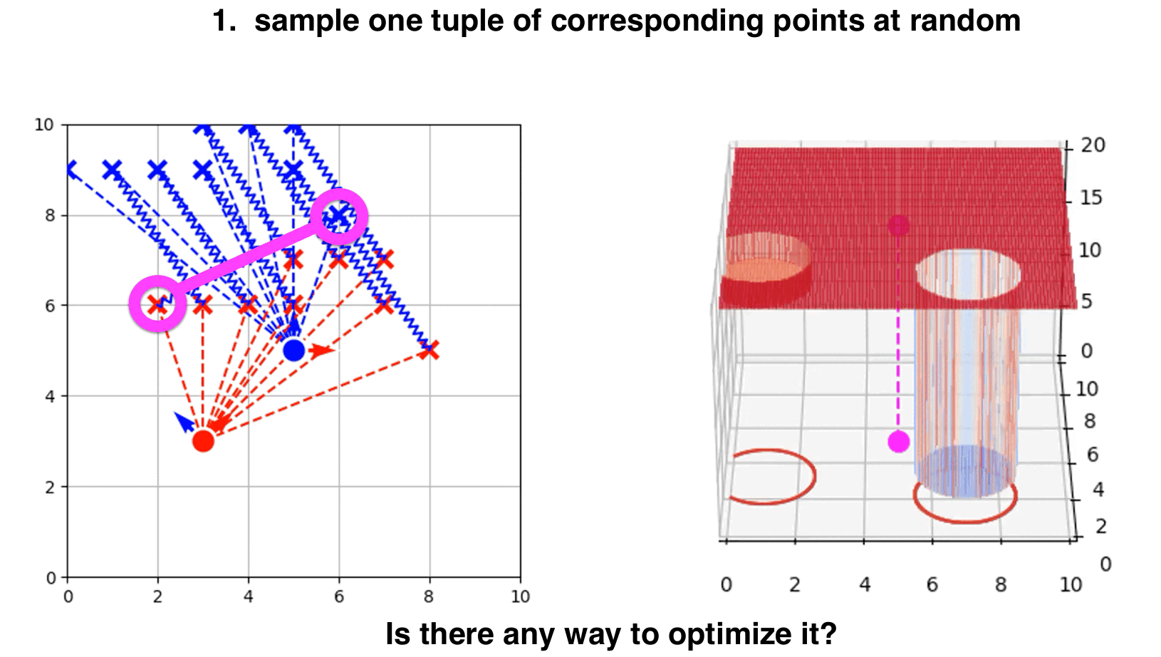
This example shows optimization on correctly matched tuples of points with L2 norm.
However, challenges arise when the matching process results in incorrect matches, commonly referred to as outliers. Such inaccuracies can cause substantial errors in the estimated transformation between point clouds, leading to misalignments in the ICP results.
Recall that so far a variant of the IPC algorithm, utilises the L2 loss function. This particular loss function is highly sensitive to incorrect matches, especially when the matched points are significantly distant from each other in reality.
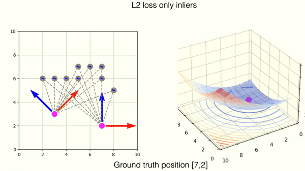
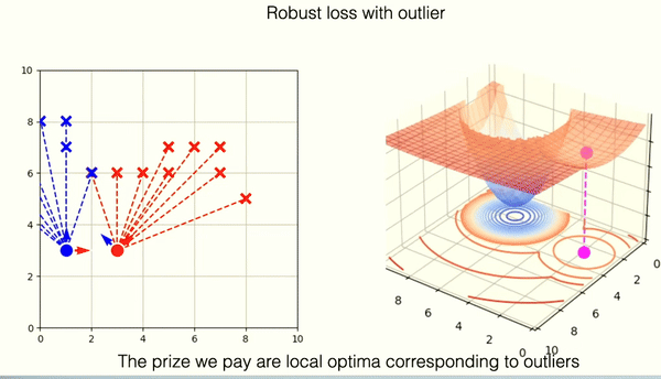
This example shows optimization on incorrectly matched tuples of points with L2 norm. One outlier is responsible for deviation from the correct position.
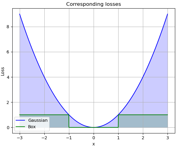
To tackle this problem, we can utilize so-called Robust loss functions that try to mitigate, the impact of outliers on the optimization process of ICP. These functions are designed to mitigate the impact of outliers on the overall performance of the algorithm. The fundamental problem with the L2 norm is that the loss increases quadratically with the distance between two matched points. In instances of incorrect matching, it is preferable for the loss to plateau or at least not increase exponentially after a certain threshold distance.
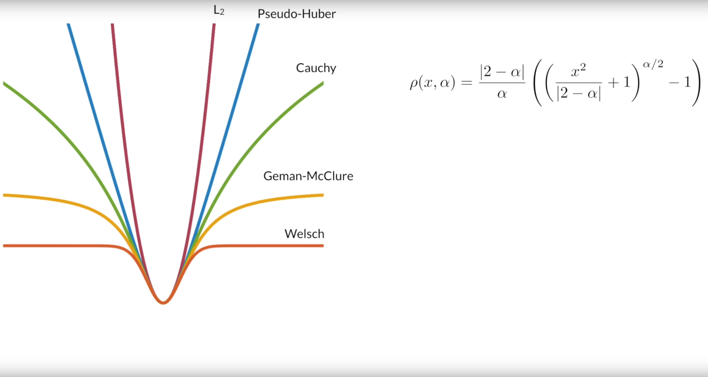
Different examples of robust loss functions. The shape of the loss function is determined by the parameter $\alpha$. For $\alpha = 2$ we get the classic L2 norm and for $\alpha = \infty$ we get Welsch loss which corresponds to the heavy-trailed Gaussian loss. Courtesy of [A General and Adaptive Robust Loss Function](https://arxiv.org/abs/1701.03077).
We can utilize so-called, heavy-tailed Gaussian, which is a combination of uniform and Gaussian probability distribution. The loss function of heavy-trailed Gaussian can be adjusted to be more forgiving for distant, incorrect matches, thereby enhancing the robustness of the ICP algorithm in handling outliers and improving its overall accuracy.
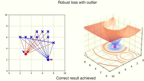
The robust loss successfully mitigates the wrong match. You can observe, however, that the loss landscape contains one new local minima. This corresponds to the wrong matching solution.
Drawbacks of robust loss functions
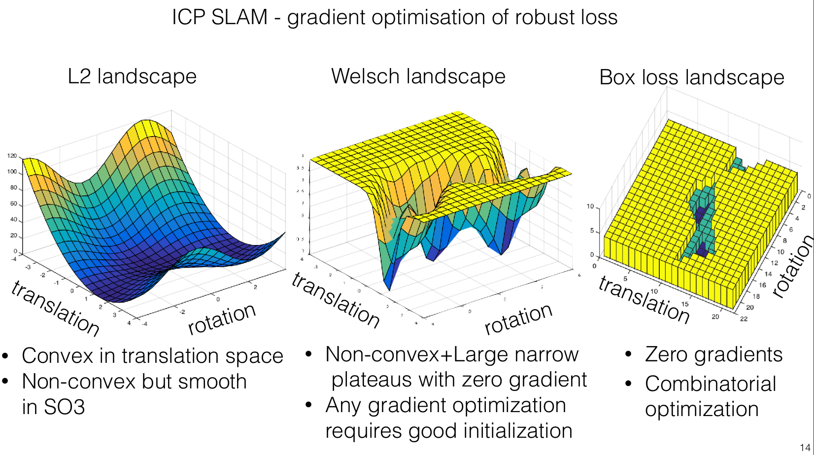
The primary advantage of the L2 loss function lies in the simplicity of its optimization, which is reflected in its gradient landscape. The L2 loss results in a convex gradient landscape where the path to the global optimum is straightforward and predictable.
In contrast, the gradient landscape of a heavy-tailed Gaussian loss function is more complex. This landscape is characterized by a larger area of low gradients, which can slow the convergence rate as the algorithm may not be propelled strongly toward the optimum by the gradient. Moreover, this type of landscape is more prone to local optima—areas where the gradient is minimal or zero but which do not represent the best possible solution globally. The local optima are in most cases areas of incorrect solutions of the ICP algorithm.
RANSAC-like optimization using Box Loss
The disadvantage of local optima for robust loss functions sparked an idea to replace the loss function with the so-called box loss function. This function is characterized by having gradients that are either zero or undefined.
You can also imagine box loss as a function that counts the number of outliers.
Given the gradient-less characteristics of the box loss function, traditional gradient-based optimization methods cannot be used. Instead, an alternative approach involves searching for the appropriate transformation directly. This leads us to a method similar to the RANSAC algorithm, which is effective in handling scenarios with a significant amount of outliers or noise.
This adapted algorithm works by randomly selecting pairs of points from reference and sensor point clouds, and then determining the transformation that minimizes the distance between these matched points. The process of the algorithm includes the following steps:
Algorithm
- Repeat the following steps for a fixed number of iterations:
- Randomly select a subset of points from the reference and sensor point clouds. The subset size is determined by the problem we are trying to solve. In this case, we are only looking for the translation of point clouds and not rotation. Therefore only one tuple of points is enough.
- Compute the transformation (translation) between the selected points.
- Align the point clouds using the computed transformation.
- Translate the point clouds and count the number of inlier points.
- Keep track of the transformation with the highest number of inliers.
- Return the best transformation as a result.
RANSAC-like ICP step by step.
Example 1: Translation and rotation
To estimate translation and rotation accurately using this RANSAC-like algorithm with the box loss function, we need to sample at least two pairs of correspondences. This minimum requirement allows for the computation of both rotation and translation parameters by aligning these point pairs. Here’s how the process unfolds:
How many times should I sample the hypothesis?
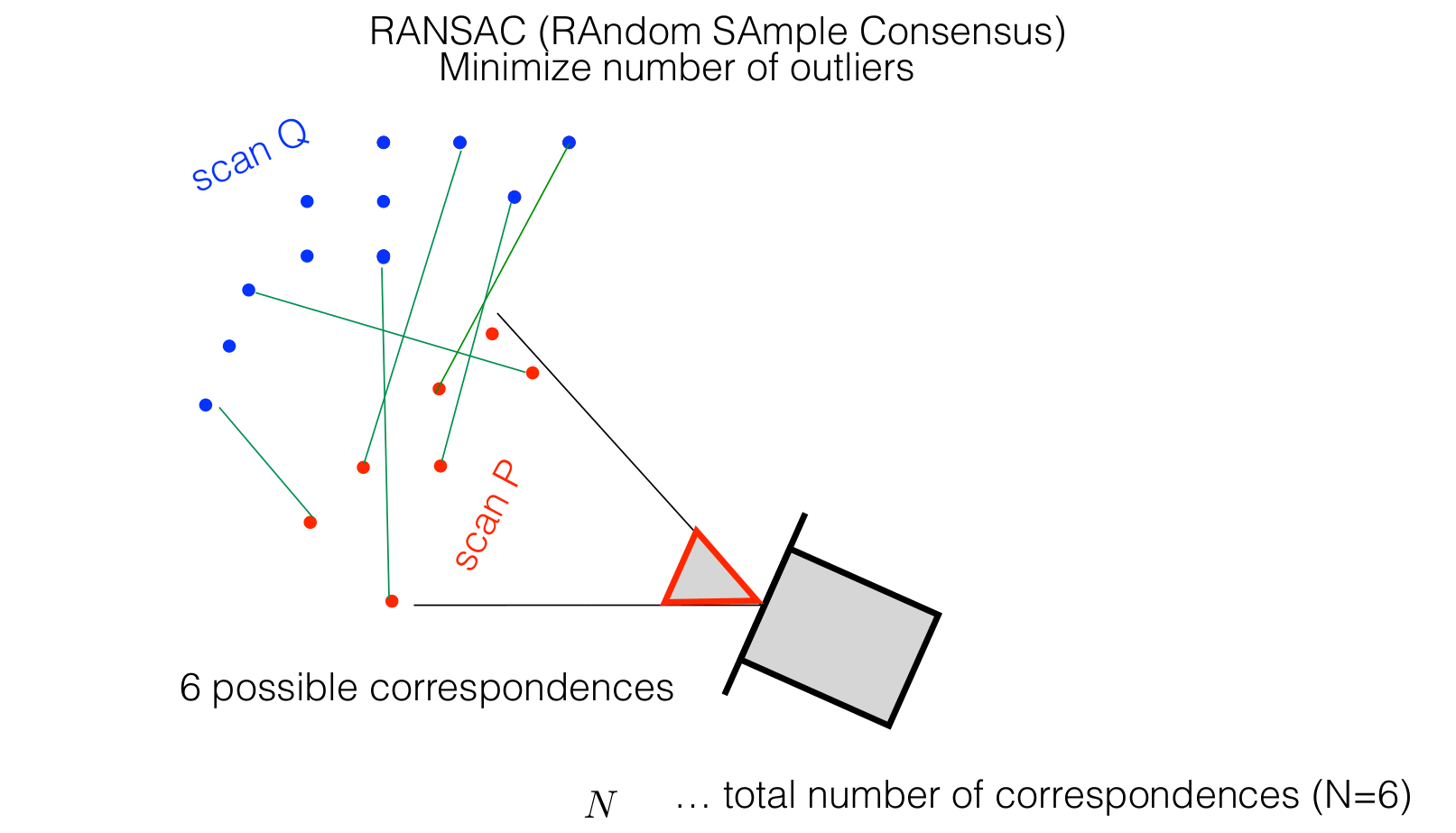
The RANSAC (Random Sample Consensus) algorithm is designed to robustly estimate model parameters from datasets contaminated with outliers. It accomplishes this by iteratively selecting a random subset of data points, fitting a model to these points, and evaluating the model’s validity against the entire dataset.
To ensure a high probability of successfully identifying a subset composed solely of inliers, RANSAC relies on a specific formula to determine the minimal number of iterations (K) required:
\[K = \frac{\log{(1-p)}}{\log{(1-w^s)}}\]Here’s a breakdown of the parameters used in this formula:
- $p$: The desired probability of success, often set close to 1 (e.g., 0.99), representing a 99% confidence level that the algorithm will select at least one inlier-only subset during its iterations.
- $w$: Ratio of inliers.
- $s$: Number of data points sampled in each iteration. This number is determined by the model that is being fitted.
Summary
- Even though the minimization of L2 loss is fairly straightforward, outlier correspondences heavily affect the result. Minimization with outliers produces biased point cloud alignment.
- Robust norms attempt to address this by limiting the effect of distant correspondences. However, optimizing these functions is more complicated due to minimal gradients and local optima. Therefore, we need to ensure that we are initializing the algorithm close to the global optimum (high frequency of ICP).
- In cases where we cannot run the ICP algorithm with high frequency, i.e., the motion between two scans is too large, we can utilize a RANSAC-like method. This method randomly samples a hypothesis $K$ times and selects the hypothesis with the highest number of inliers. RANSAC methods are commonly used for matching image correspondences.
Additional materials
This video briefly explains robust loss functions, with some nice animations. In case you are interested, in how could these loss functions look in state-of-the-art SLAM algorithms, you can check out the documentation for libpointmatcher library here.
Author: Michal Kasarda